





Author: Parth Rana
Affiliation: Stern Group, Department of Physics and Astronomy, Northwestern University
This notebook is associated with the publication Magnetic Proximity Coupling in Valley Exciton-Polaritons by Garvey et al.
Obliquely incident circularly polarized light resonating in an optical microcavity can deviate from pure circular polarization due to the different Fresnel reflection coefficients of s- and p-polarized light. We investigate this effect in a particular optical microcavity developed in the above publication, as many measurements reported in the manuscript involve valley-selective excitation of the monolayer WSe2 embedded within the cavity. Selective coupling to a particular valley requires highly circularly polarized light, so it is important to verify that light resonating in the cavity remains largely circularly polarized and that valley-selective coupling is therefore not compromised.
In this notebook, we examine this by sweeping wavelength and incident angle for circularly polarized light incident on the cavity and then analyzing the polarization of the intracavity field.
Simulation Setup
We begin by constructing a simulated microcavity designed to model the real experimental microcavity associated with the above publication. First, materials used in the cavity were defined, including Si3N4, SiO2, Al2O3, and Ag. Each material was modeled with the pole-residue model using material data from the Tidy3D library.
import tidy3d as td
import numpy as np
import tidy3d.web as web

# Suppress warnings for field decay warnings
td.config.logging.level = "ERROR"

# Materials used in the cavity. Material models and source references are specified in the variable names.

Vacuum = td.Medium(
    name = 'Vacuum',
)

Silicon_Nitride___Si3N4___Philipp1973Sellmeier = td.PoleResidue(
    name = 'Silicon Nitride ("Si3N4")_Philipp1973Sellmeier',
    frequency_range = [241768111758828.06, 1448272746767859],
    poles = [[(0 + 13486443552366650j), (0-19514209498096924j)]]
)

SiO2_Malitson_1965 = td.PoleResidue(
    name = 'SiO2_Malitson-1965',
    frequency_range = [44745142985074.625, 1427583133333333.5],
    eps_inf = 1.3040957096247774,
    poles = [[(-0.010768524680114307-190296337851301.47j), (0.0022707553833665978 + 85470898621396.69j)], [(-4.3854868234548885-18045696608255308j), (3.200090437230946 + 7218959877530578j)]]
)

Al2O3_Malitson = td.PoleResidue(
    name = 'Al2O3_Malitson',
    frequency_range = [59958491600000, 1498962290000000],
    poles = [[(-23434.288815096003-25916678071049150j), (134.11731758468494 + 18553587289566490j)], [(-4683.69992744982-15785324390464258j), (15272.289190111514 + 5131079251364668j)], [(-4.827979986277954-104483267274091.89j), (0 + 279042282535100.44j)]]
)

Silver___Ag___JohnsonChristy1972 = td.PoleResidue(
    name = 'Silver ("Ag")_JohnsonChristy1972',
    frequency_range = [154771532566312.25, 1595489401708072.2],
    poles = [[(-2208321413508536-5948722238054062j), (6900545964172845 + 2859999298140436j)], [(-454071262600809.06-6045413448570748j), (900170460600995-571876746089699.8j)], [(-440069917626400.94-1501005120704881.8j), (-624427112339892.1-709709047591569.2j)], [(-90645222183131.28-1207503089909680.2j), (36466030087984.664-105435949158129.28j)], [(-6882166770889.508-101422373698470.4j), (2204704963300273.8 + 925991991669040600j)]]
)
Next, the overall structure of the cavity was constructed. The cavity consists of two mirrors: a top silver mirror and a bottom Distributed-Bragg Reflector (DBR) composed of alternating Si3N4 and SiO2 layers. The cavity spacer is made of Al2O3.
It is worth noting that there are some differences in the simulated structure compared to the real experimental cavity. Tidy3D is a classical electromagnetic solver, so atomically thin layers of WSe2 and CrI3 embedded in the real cavity were not added. These layers are important for the quantum exciton-polariton behavior of the experimental system, but the goal of this simulation was instead to study the classical polarization response of light resonating in the cavity.
Additionally, to make the simulated cavity match the experimental structure as closely as possible, the Al2O3 spacer and top Ag mirror thicknesses were tuned so the simulated reflectance spectrum reproduced the experimental resonant wavelength and linewidth. Although that simulation is not shown here, it determined the final Al2O3 spacer and Ag mirror thicknesses to be 172.908 nm and 13.650 nm, respectively.
#Structures used to construct the cavity

#Top Mirror (Ag)
Silver_Mirror = td.Structure(
    geometry = td.Box(center = [0, 0, 0.225133], size = [td.inf * 0.001, td.inf * 0.001, 0.01365]),
    name = 'Silver Mirror',
    medium = Silver___Ag___JohnsonChristy1972
)

#Cavity Spacer (Al2O3)
Cavity = td.Structure(
    geometry = td.Box(center = [0, 0, 0.13185400000000003], size = [td.inf * 0.001, td.inf * 0.001, 0.17290799999999998]),
    name = 'Cavity',
    medium = Al2O3_Malitson
)

#Bottom Mirror (10 Pair DBR alternating SiO2 and Si3N4 with a terminating layer of Si3N4)
Pair1_Si3N4 = td.Structure(
    geometry = td.Box(size = [td.inf, td.inf, 0.09079999999999999]),
    name = 'Pair1-Si3N4',
    medium = Silicon_Nitride___Si3N4___Philipp1973Sellmeier
)

Pair1_SiO2 = td.Structure(
    geometry = td.Box(center = [0, 0, -0.10784999999999999], size = [td.inf * 0.001, td.inf * 0.001, 0.12490000000000001]),
    name = 'Pair1-SiO2',
    medium = SiO2_Malitson_1965
)

Pair2_Si3N4 = td.Structure(
    geometry = td.Box(center = [0, 0, -0.21569999999999998], size = [td.inf, td.inf, 0.09079999999999999]),
    name = 'Pair2-Si3N4',
    medium = Silicon_Nitride___Si3N4___Philipp1973Sellmeier
)

Pair2_SiO2 = td.Structure(
    geometry = td.Box(center = [0, 0, -0.32355], size = [td.inf * 0.001, td.inf * 0.001, 0.12490000000000001]),
    name = 'Pair2-SiO2',
    medium = SiO2_Malitson_1965
)

Pair3_Si3N4 = td.Structure(
    geometry = td.Box(center = [0, 0, -0.43139999999999995], size = [td.inf, td.inf, 0.09079999999999999]),
    name = 'Pair3-Si3N4',
    medium = Silicon_Nitride___Si3N4___Philipp1973Sellmeier
)

Pair3_SiO2 = td.Structure(
    geometry = td.Box(center = [0, 0, -0.53925], size = [td.inf * 0.001, td.inf * 0.001, 0.12490000000000001]),
    name = 'Pair3-SiO2',
    medium = SiO2_Malitson_1965
)

Pair4_Si3N4 = td.Structure(
    geometry = td.Box(center = [0, 0, -0.6471], size = [td.inf, td.inf, 0.09079999999999999]),
    name = 'Pair4-Si3N4',
    medium = Silicon_Nitride___Si3N4___Philipp1973Sellmeier
)

Pair4_SiO2 = td.Structure(
    geometry = td.Box(center = [0, 0, -0.75495], size = [td.inf * 0.001, td.inf * 0.001, 0.12490000000000001]),
    name = 'Pair4-SiO2',
    medium = SiO2_Malitson_1965
)

Pair5_Si3N4 = td.Structure(
    geometry = td.Box(center = [0, 0, -0.8627999999999999], size = [td.inf, td.inf, 0.09079999999999999]),
    name = 'Pair5-Si3N4',
    medium = Silicon_Nitride___Si3N4___Philipp1973Sellmeier
)

Pair5_SiO2 = td.Structure(
    geometry = td.Box(center = [0, 0, -0.97065], size = [td.inf * 0.001, td.inf * 0.001, 0.12490000000000001]),
    name = 'Pair5-SiO2',
    medium = SiO2_Malitson_1965
)

Pair6_Si3N4 = td.Structure(
    geometry = td.Box(center = [0, 0, -1.0785], size = [td.inf, td.inf, 0.09079999999999999]),
    name = 'Pair6-Si3N4',
    medium = Silicon_Nitride___Si3N4___Philipp1973Sellmeier
)

Pair6_SiO2 = td.Structure(
    geometry = td.Box(center = [0, 0, -1.18635], size = [td.inf * 0.001, td.inf * 0.001, 0.12490000000000001]),
    name = 'Pair6-SiO2',
    medium = SiO2_Malitson_1965
)

Pair7_Si3N4 = td.Structure(
    geometry = td.Box(center = [0, 0, -1.2942], size = [td.inf, td.inf, 0.09079999999999999]),
    name = 'Pair7-Si3N4',
    medium = Silicon_Nitride___Si3N4___Philipp1973Sellmeier
)

Pair7_SiO2 = td.Structure(
    geometry = td.Box(center = [0, 0, -1.40205], size = [td.inf * 0.001, td.inf * 0.001, 0.12490000000000001]),
    name = 'Pair7-SiO2',
    medium = SiO2_Malitson_1965
)

Pair8_Si3N4 = td.Structure(
    geometry = td.Box(center = [0, 0, -1.5099], size = [td.inf, td.inf, 0.09079999999999999]),
    name = 'Pair8-Si3N4',
    medium = Silicon_Nitride___Si3N4___Philipp1973Sellmeier
)

Pair8_SiO2 = td.Structure(
    geometry = td.Box(center = [0, 0, -1.61775], size = [td.inf * 0.001, td.inf * 0.001, 0.12490000000000001]),
    name = 'Pair8-SiO2',
    medium = SiO2_Malitson_1965
)

Pair9_Si3N4 = td.Structure(
    geometry = td.Box(center = [0, 0, -1.7255999999999998], size = [td.inf, td.inf, 0.09079999999999999]),
    name = 'Pair9-Si3N4',
    medium = Silicon_Nitride___Si3N4___Philipp1973Sellmeier
)

Pair9_SiO2 = td.Structure(
    geometry = td.Box(center = [0, 0, -1.83345], size = [td.inf * 0.001, td.inf * 0.001, 0.12490000000000001]),
    name = 'Pair9-SiO2',
    medium = SiO2_Malitson_1965
)

Pair10_Si3N4 = td.Structure(
    geometry = td.Box(center = [0, 0, -1.9413], size = [td.inf, td.inf, 0.09079999999999999]),
    name = 'Pair10-Si3N4',
    medium = Silicon_Nitride___Si3N4___Philipp1973Sellmeier
)

Pair10_SiO2 = td.Structure(
    geometry = td.Box(center = [0, 0, -2.04915], size = [td.inf * 0.001, td.inf * 0.001, 0.12490000000000001]),
    name = 'Pair10-SiO2',
    medium = SiO2_Malitson_1965
)

Pair11_Si3N4 = td.Structure(
    geometry = td.Box(center = [0, 0, -2.157], size = [td.inf, td.inf, 0.09079999999999999]),
    name = 'Pair11-Si3N4',
    medium = Silicon_Nitride___Si3N4___Philipp1973Sellmeier
)
In order to measure the electromagnetic field dynamics, several field time monitors were used. The first four monitors were placed above the structure to measure the polarization of the reflected light, while the other two monitors were placed inside the cavity to measure the intracavity polarization.
# Monitors for EM field with respect to time
mon1 = td.FieldTimeMonitor(
    name = '(0, 0) fieldtimemonitor',
    center = [0, 0, 2.2],
    size = [0, 0, 0],
    interval = 1
)

mon2 = td.FieldTimeMonitor(
    name = '(0.25, 0) fieldtimemonitor',
    center = [-0.25, 0, 2.2],
    size = [0, 0, 0],
    interval = 1
)

mon3 = td.FieldTimeMonitor(
    name = '(0.5, 0) fieldtimemonitor',
    center = [-0.5, 0, 2.2],
    size = [0, 0, 0],
    interval = 1
)

mon4 = td.FieldTimeMonitor(
    name = '(0.75, 0) fieldtimemonitor',
    center = [-0.75, 0, 2.2],
    size = [0, 0, 0],
    interval = 1
)

mon5 = td.FieldTimeMonitor(
    name = '(0, 0) CAVITY-fieldtimemonitor',
    center = [0, 0, 0.13186],
    size = [0, 0, 0],
    interval = 1
)

mon6 = td.FieldTimeMonitor(
    name = '(0.5, 0) CAVITY-fieldtimemonitor',
    center = [-0.5, 0, 0.13186],
    size = [0, 0, 0],
    interval = 1
)
Since Tidy3D does not provide a built-in circularly polarized source option, circular polarization was simulated using two separate plane-wave simulations. The first used a linearly p-polarized source, and the second used a linearly s-polarized source with a 90° phase shift. By superimposing the results of these simulations, the interaction of circularly polarized light with the structure could be reconstructed.
So, a simulation object was defined depending on the incident wavelength, angle, and polarization. Various incident angles were swept between 0° and 25°, and wavelengths were swept between 660 nm and 740 nm. In general, the wavelengths were swept in 10 nm increments, except around the resonant wavelength where additional data points were taken. Investigating polarization near the resonance is particularly important as this is where the polarization is expected to deviate most strongly from purely circular behavior. Near resonance, repeated internal reflections within the cavity cause small differences between the s- and p-polarized components to accumulate, leading to larger differences in reflectivity and therefore greater deviations from circular polarization.
However, the resonant wavelength of a cavity also depends on incident angle. Therefore, to identify the resonant wavelength, preliminary simulations not shown here were performed to obtain the reflectance spectrum of the cavity at every incident angle, similar to the thickness-tuning simulation discussed above. The results of these simulations informed the wavelength values chosen in wsweeps_by_angle, ensuring that additional simulations were performed near resonance at each angle.
To finish, boundary conditions and runtime were specified. Bloch boundary conditions were applied in the x and y directions, while perfectly matched layers (PMLs) were used in the z direction. The runtime was set to 1 picosecond, and a field monitor was added to visualize the electromagnetic field within the structure.
# Angles being swept
angle_sweeps = np.array([0, 5, 10, 12, 15, 17.5, 20, 22.5, 23.75, 25])

# Polarizations being swept
polarization_sweeps = ["s", "p"]

# s-polarization normalization constants by incident angle (control simulations showed that the two polarizations were not balanced in magnitude)
s_norm_by_angle = {
    0 : 1.00,
    5 : 0.999698088,
    10 : 0.99885452,
    12 : 0.998409049,
    15 : 0.99765978,
    17.5 : 0.997010118,
    20 : 0.996376407,
    22.5 : 0.995798026,
    23.75 : 0.995544533,
    25 : 0.99532944
}

# Wavelength sweeps in microns, organized by incident angle
wsweeps_by_angle = {
    0: np.array([
        0.660, 0.670, 0.680, 0.690, 0.700,
        0.710, 0.720, 0.730, 0.740
    ]),

    5: np.array([
        0.660, 0.670, 0.680, 0.690, 0.700, 0.710,
        0.715, 0.71663, 0.71827, 0.71913, 0.720,
        0.72163, 0.725, 0.730, 0.740
    ]),

    10: np.array([
        0.660, 0.670, 0.680, 0.690, 0.700, 0.710,
        0.712639, 0.714139, 0.715789, 0.716239,
        0.716639, 0.717489, 0.719139, 0.720639,
        0.730, 0.740
    ]),

    12: np.array([
        0.660, 0.670, 0.680, 0.690, 0.700, 0.710,
        0.711101, 0.712301, 0.713401, 0.714251,
        0.714701, 0.715101, 0.715951, 0.716801,
        0.717901, 0.719101, 0.720, 0.730, 0.740
    ]),

    15: np.array([
        0.660, 0.670, 0.680, 0.690, 0.700,
        0.708977, 0.710477, 0.712127, 0.712977,
        0.713827, 0.715477, 0.716977, 0.720,
        0.730, 0.740
    ]),

    17.5: np.array([
        0.660, 0.670, 0.680, 0.690, 0.700,
        0.70595, 0.70745, 0.7091, 0.70955,
        0.70995, 0.7108, 0.71245, 0.71395,
        0.720, 0.730, 0.740
    ]),

    20: np.array([
        0.660, 0.670, 0.680, 0.690, 0.700,
        0.703007, 0.704507, 0.706157, 0.706607,
        0.707007, 0.707857, 0.709507, 0.711007,
        0.720, 0.730, 0.740
    ]),

    22.5: np.array([
        0.660, 0.670, 0.680, 0.690,
        0.699863, 0.701363, 0.703013, 0.703463,
        0.703863, 0.704713, 0.706363, 0.707863,
        0.710, 0.720, 0.730, 0.740
    ]),

    23.75: np.array([
        0.660, 0.670, 0.680, 0.690,
        0.697124, 0.698374, 0.699624, 0.700624,
        0.701274, 0.701724, 0.702124, 0.702974,
        0.704624, 0.705874, 0.707124,
        0.710, 0.720, 0.730, 0.740
    ]),

    25: np.array([
        0.660, 0.670, 0.680, 0.690, 0.695,
        0.6964, 0.697472, 0.6981, 0.698972,
        0.69962, 0.70022, 0.700622, 0.701472,
        0.702322, 0.703972, 0.705472,
        0.710, 0.720, 0.730, 0.740
    ])
}


## make_sim: makes one Tidy3D simulation for a given:
##    wl        wavelength in microns
##    angle_deg incident angle in degrees
##    pol       "s" or "p"
def make_sim(wl, angle_deg, pol):
    if pol == "s":
        amplitude = s_norm_by_angle[angle_deg]   # amplitude was used to normalize s-polarization sims to match p-polarization sims
        phase = np.pi / 2   # Pi/2 phase was used for s-polarization sims
        pol_angle = np.pi / 2   # Sets s-polarization

    elif pol == "p":
        amplitude = 1.0
        phase = 0.0    # 0 phase was used for p-polarization sims
        pol_angle = 0.0   # Sets p-polarization

    planewave = td.PlaneWave(
        name = 'planewave',
        center = [0, 0, 2],
        size = [td.inf, td.inf, 0],
        source_time = td.ContinuousWave(amplitude = amplitude, phase = phase, freq0 = td.C_0/wl, fwidth = 14449493712968.438),
        direction = '-',
        angle_theta = np.deg2rad(angle_deg), # This is the incident angle
        pol_angle = pol_angle
    )

    #Field monitor to visualize field, dependent on incident wavelength used in simulation
    fieldmonitor = td.FieldMonitor(
        name = 'fieldmonitor_15',
        size = [td.inf, 0, 4.5],
        freqs = td.C_0 / wl,
    )

    #Bloch boundaries that match PlaneWave angles + freq
    bx = td.BlochBoundary.from_source(
        source=planewave,
        domain_size=2.0,
        axis=0,
        medium=Vacuum
    )

    by = td.BlochBoundary.from_source(
        source=planewave,
        domain_size=2.0,
        axis=1,
        medium=Vacuum
    )

    sim = td.Simulation(
        center = [0, 0, -0.2],
        size = [2, 2, 5.4],
        normalize_index = None,
        boundary_spec = td.BoundarySpec(x = td.Boundary(plus = bx, minus = bx), y = td.Boundary(plus = by, minus = by), z = td.Boundary(plus = td.PML(), minus = td.PML())),
        grid_spec = td.GridSpec(grid_x = td.AutoGrid(min_steps_per_wvl = 11), grid_y = td.AutoGrid(min_steps_per_wvl = 11), grid_z = td.AutoGrid(min_steps_per_wvl = 11)),
        run_time = 1e-12,
        medium = Vacuum,
        sources = [planewave],
        monitors = [mon1, mon2, mon3, mon4, mon5, mon6, fieldmonitor],
        structures = [Pair1_Si3N4, Pair1_SiO2, Pair2_Si3N4, Pair2_SiO2, Pair3_Si3N4, Pair3_SiO2, Pair4_Si3N4, Pair4_SiO2, Pair5_Si3N4, Pair5_SiO2, Pair6_Si3N4, Pair6_SiO2, Pair7_Si3N4, Pair7_SiO2, Pair8_Si3N4, Pair8_SiO2, Pair9_Si3N4, Pair9_SiO2, Pair10_Si3N4, Pair10_SiO2, Pair11_Si3N4, Cavity, Silver_Mirror]
    )

    return sim
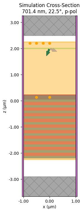
After all the components of the simulation were defined, the full batch of simulations was run across a range of incident angles, wavelengths, and the two polarizations. Below is a cross section of what a single simulation would look like, with this example being for 701.363 nm p-polarized light at 22.5° incidence:
import matplotlib.pyplot as plt

# Plotting one simulation as example:
test_wl = 0.701363
test_angle = 22.5
test_pol = "p"

test_sim = make_sim(test_wl, test_angle, test_pol)
fig, ax = plt.subplots(figsize=(6, 8))

#x-z plane cross section
test_sim.plot(
    y=0.0,
    ax=ax
)

ax.set_title(
    f"Simulation Cross-Section\n"
    f"{test_wl*1e3:.1f} nm, {test_angle}°, {test_pol}-pol"
)

plt.show()
sims = {}

for angle_deg in angle_sweeps:
    for wl in wsweeps_by_angle[angle_deg]:
        for pol in polarization_sweeps:
            sim_name = f"angle={angle_deg:g}deg_wl={wl*1e3:.3f}nm_{pol}"
            sims[sim_name] = make_sim(wl, angle_deg, pol)


batch = web.Batch(simulations=sims, verbose=True)
batch_results = batch.run(path_dir="angle/wl_results")
Output()
10:02:36 EDT Started working on Batch containing 322 tasks.
10:07:37 EDT Maximum FlexCredit cost: 65.693 for the whole batch.
             Use 'Batch.real_cost()' to get the billed FlexCredit cost after
             completion.
Output()
10:10:15 EDT Batch complete.
Data Analysis and Results
After running these simulations, the field time monitors had accumulated lots of electromagnetic field data over time for many wavelengths and incident angles. The goal was then to determine the steady-state polarization inside the cavity for each of these wavelengths and incident angles. To do that, the total polarization was reconstructed using the linear polarization simulation results.
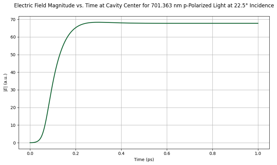
First, a time segment was chosen from which to extract the polarization data. For all simulations, this segment was taken at 0.9 ps after the start of the simulation. As shown clearly in the electric field magnitude plot below for one of the simulations, this time lies well after the system had reached steady state, as indicated by the asymptotic behavior of the field magnitude.
import numpy as np
import matplotlib.pyplot as plt
import math
import pandas as pd
from pathlib import Path

plot_angle = 22.5
plot_wl = 0.701363
plot_pol = "p"

sim_name = f"angle={plot_angle:g}deg_wl={plot_wl*1e3:.3f}nm_{plot_pol}"
sim_data = batch_results[sim_name]

time_monitor_name = "(0, 0) CAVITY-fieldtimemonitor"   # CHANGE THIS if your center cavity monitor has a different name

time_data = sim_data[time_monitor_name]

Ex = time_data.Ex
Ey = time_data.Ey
Ez = time_data.Ez

# Electric field magnitude
E_mag = np.sqrt(np.abs(Ex)**2 + np.abs(Ey)**2 + np.abs(Ez)**2).squeeze()

# Time coordinate
t = E_mag.coords["t"].values

fig, ax = plt.subplots(figsize=(9, 5.5))
ax.plot(t * 1e12, E_mag.values, linewidth=2)

ax.set_xlabel("Time (ps)")
ax.set_ylabel(r"$|E|$ (a.u.)")
ax.set_title(
    f"Electric Field Magnitude vs. Time at Cavity Center for 701.363 nm p-Polarized Light at 22.5° Incidence\n"
)

ax.grid(True)
plt.tight_layout()
plt.show()
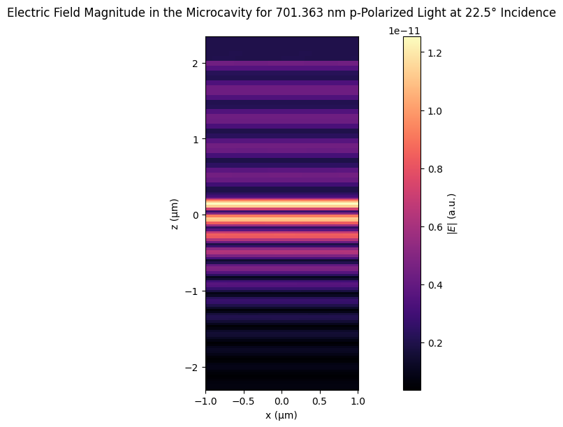
The next figure below shows the spatial distribution of the steady-state electric field magnitude. As expected, the electric field inside the cavity is much stronger than anywhere else in the structure (cavity location is indicated by the first, brightest band at z ≈ 0.2um). The field becomes much weaker farther down into the DBR, consistent with the expected reflective behavior of the DBR.
s = sim_data._get_scalar_field(
    field_monitor_name="fieldmonitor_15",
    field_name="E",
    val="abs"
)

f0 = td.C_0 / plot_wl
plot_data = s.sel(y=0, f=f0, method="nearest")

x = plot_data["x"].values
z = plot_data["z"].values
E = plot_data.values

fig, ax = plt.subplots(figsize=(8, 6), constrained_layout=True)
im = ax.pcolormesh(x, z, E.T, shading="auto", cmap="magma")

ax.set_xlabel("x (μm)")
ax.set_ylabel("z (μm)")
ax.set_title(f"Electric Field Magnitude in the Microcavity for 701.363 nm p-Polarized Light at 22.5° Incidence\n")

ax.set_aspect("equal")
cbar = fig.colorbar(im, ax=ax)
cbar.set_label(r"$|E|$ (a.u.)")

plt.show()
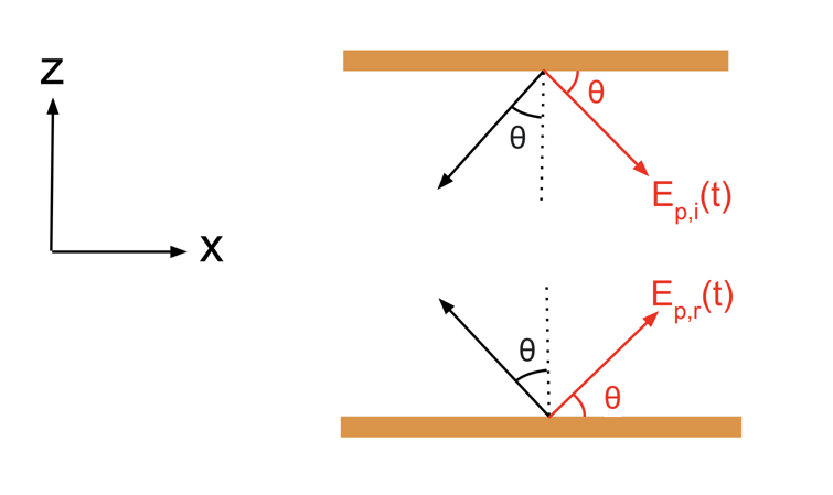
Reconstructing the exact degree of circular polarization inside the cavity requires a bit of geometric thinking. When the propagation direction of the incident light is angled, the incident p-polarization component ${E_{p,i}}$ is likewise angled within the x-z plane, making an angle $\theta$ to the x-axis where $\theta$ is the same as the angle of incidence. Consequently, by the law of reflection, the reflected p-polarization component ${E_{p,r}}$ is obtained by reflecting the incident component ${E_{p,i}}$ across the x-axis:
The quantity of interest is the combined p-polarized amplitude inside the cavity, ${E_p(t)}$, so that it can be plotted against ${E_s(t)}$. If we assume that the incident and reflected p-polarization components shown above are the only relevant p-polarization directions present in the cavity, then we define ${E_p(t)} \equiv {E_{p,i}(t)} + {E_{p,r}(t)}$. It is worth noting that ${E_p(t)}$ is not the magnitude of the net p-polarized field. The field-time monitor records the net electric field in Cartesian coordinates, $\mathbf{E}(t) = E_x(t)\hat{x} + E_z(t)\hat{z}$, and some basic trigonometry allows us to find ${E_p(t)}$ from the recorded $E_x(t)$:
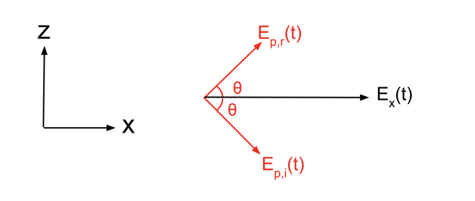
Clearly ${E_{p,i}(t)\cos\theta} + {E_{p,r}(t)\cos\theta}=E_x(t)$, so ${E_p(t)} \equiv {E_{p,i}(t)} + {E_{p,r}(t)} = E_x(t)\sec\theta$. No analogous correction is needed for the s-polarized component since ${E_s(t)}$ is entirely along the y axis regardless of the angle of incidence, and thus ${E_s(t)}=E_y(t)$.
The main assumption made in this analysis is that only the two propagation directions specified in the figures above contribute appreciably inside the cavity. We believe this is a good assumption because other simulation results indicate that the electric field of the light reflected out of the cavity is nearly perfectly aligned with the $E_{p,r}$ direction. Since this reflected light includes light that has resonated within the cavity for some time, it suggests that the propagation vector inside the cavity generally continues to obey the law of reflection to a very good approximation.
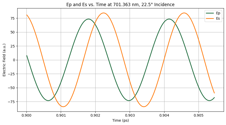
The resulting ${E_p(t)}$ and ${E_s(t)}$ are plotted below against time for the 701.363 nm at 22.5° incidence example. Electric field data for the s- and p-polarized light were analyzed starting at 0.9 ps as explained before using 300 data points with a time step of $1.82 \times 10^{-5}$ picoseconds.
# -------------------------
# Extract Ep and Es
# -------------------------

def get_ep_es_from_batch(
    batch_results,
    angle_deg,
    wl_um,
    monitor_name="(0, 0) CAVITY-fieldtimemonitor",
    x0=0,
    y0=0,
    z0=0.13186,
    t_start_ps=0.9,
    n_samples=300,
):

    sim_name_p = f"angle={angle_deg:g}deg_wl={wl_um*1e3:.3f}nm_p"
    sim_name_s = f"angle={angle_deg:g}deg_wl={wl_um*1e3:.3f}nm_s"

    sim_data_p = batch_results[sim_name_p]
    sim_data_s = batch_results[sim_name_s]

    mon_p = sim_data_p[monitor_name]
    mon_s = sim_data_s[monitor_name]

    # Extract Data
    Ex_da = mon_p.Ex.sel(x=x0, y=y0, z=z0)
    Ey_da = mon_s.Ey.sel(x=x0, y=y0, z=z0)

    t_p = np.array(Ex_da.t.values, dtype=float)
    t_s = np.array(Ey_da.t.values, dtype=float)

    Ex = np.real(Ex_da.values)
    Ey = np.real(Ey_da.values)

    t_start_s = t_start_ps * 1e-12

    start_idx_p = np.searchsorted(t_p, t_start_s, side="left")
    start_idx_s = np.searchsorted(t_s, t_start_s, side="left")

    end_idx_p = start_idx_p + n_samples
    end_idx_s = start_idx_s + n_samples

    # Slice the first 300 samples starting at t >= 0.9 ps
    t_p = t_p[start_idx_p:end_idx_p]
    Ex = Ex[start_idx_p:end_idx_p]
    Ey = Ey[start_idx_s:end_idx_s]

    # Construct Ep and Es
    theta = np.deg2rad(angle_deg)
    Ep = Ex / np.cos(theta)
    t_ps = t_p * 1e12 # Convert time to ps for plotting
    Es = Ey

    return Ep, Es, t_ps

# ----------------------------------------------------------
# Example: Plotting Ep and Es vs. Time for 701.363nm, 22.5°
# ----------------------------------------------------------
plot_angle = 22.5
plot_wl = 0.701363

Ep, Es, t_ps = get_ep_es_from_batch(
    batch_results=batch_results,
    angle_deg=plot_angle,
    wl_um=plot_wl,
)

plt.figure(figsize=(9, 5))
plt.plot(t_ps, Ep, label="Ep", linewidth=2)
plt.plot(t_ps, Es, label="Es", linewidth=2)

plt.xlabel("Time (ps)")
plt.ylabel("Electric Field (a.u.)")
plt.title(f"Ep and Es vs. Time at 701.363 nm, 22.5° Incidence")
plt.legend()
plt.grid(True)
plt.tight_layout()
plt.show()
Finally, ${E_p(t)}$ and ${E_s(t)}$ were plotted against each other to reconstruct the polarization state in the cavity. Ellipses were fit using a direct linear least-squares method based on the numerically stable algorithm of Halíř and Flusser, as implemented in python by Hill. This allowed the polarization to be quantified using the ellipticity angle $\chi$, defined as $\chi=\arctan(\frac{b}{a})$ where $a$ and $b$ are the lengths of the semi-major and semi-minor axes of the polarization ellipse respectively. The ellipticity angle varies from 0° to 45° where 0° corresponds to linear polarization and 45° corresponds to perfectly circular polarization. Thus, larger values of $\chi$ indicate a more circular polarization state. For the 701.363 nm at 22.5° incidence example we have been working with, the fitted ellipse gives us $\chi$ = 32.94°:
# -------------------------------------------------------------
# Ellipse Fitting Algorithm Adopted from Halir and Flusser
# -------------------------------------------------------------

def fit_ellipse(x, y):
    D1 = np.vstack([x**2, x*y, y**2]).T
    D2 = np.vstack([x, y, np.ones(len(x))]).T

    S1 = D1.T @ D1
    S2 = D1.T @ D2
    S3 = D2.T @ D2

    T = -np.linalg.inv(S3) @ S2.T
    M = S1 + S2 @ T

    C = np.array(((0, 0, 2), (0, -1, 0), (2, 0, 0)), dtype=float)
    M = np.linalg.inv(C) @ M

    eigval, eigvec = np.linalg.eig(M)

    con = 4 * eigvec[0] * eigvec[2] - eigvec[1]**2
    ak = eigvec[:, np.nonzero(con > 0)[0]]

    return np.concatenate((ak, T @ ak)).ravel()


def cart_to_pol(coeffs):
    a = coeffs[0]
    b = coeffs[1] / 2
    c = coeffs[2]
    d = coeffs[3] / 2
    f = coeffs[4] / 2
    g = coeffs[5]

    den = b**2 - a*c

    if den > 0:
        raise ValueError("Invalid ellipse: b^2 - ac must be negative.")

    x0 = (c*d - b*f) / den
    y0 = (a*f - b*d) / den

    num = 2 * (a*f**2 + c*d**2 + g*b**2 - 2*b*d*f - a*c*g)
    fac = np.sqrt((a - c)**2 + 4*b**2)

    ap = np.sqrt(num / den / (fac - a - c))
    bp = np.sqrt(num / den / (-fac - a - c))

    if ap < bp:
        ap, bp = bp, ap
        swap_axes = True
    else:
        swap_axes = False

    r = (bp / ap)**2
    if r > 1:
        r = 1 / r

    e = np.sqrt(1 - r)

    if b == 0:
        phi = 0 if a < c else np.pi / 2
    else:
        phi = np.arctan(2*b / (a - c)) / 2
        if a > c:
            phi += np.pi / 2

    if swap_axes:
        phi += np.pi / 2

    phi = phi % np.pi

    return x0, y0, ap, bp, e, phi


def get_ellipse_pts(params, npts=100, tmin=0, tmax=2*np.pi):
    x0, y0, ap, bp, e, phi = params

    t = np.linspace(tmin, tmax, npts)

    x = x0 + ap * np.cos(t) * np.cos(phi) - bp * np.sin(t) * np.sin(phi)
    y = y0 + ap * np.cos(t) * np.sin(phi) + bp * np.sin(t) * np.cos(phi)

    return x, y

def fit_ep_es_ellipse(Ep, Es):
    coeffs = fit_ellipse(Ep, Es)
    x0, y0, ap, bp, e, phi = cart_to_pol(coeffs)
    ellipticity_angle = math.degrees(math.atan(bp / ap))

    return {
        "x0": x0,
        "y0": y0,
        "ap": ap,
        "bp": bp,
        "e": e,
        "phi": phi,
        "phi_deg": np.degrees(phi),
        "ellipticity_angle": ellipticity_angle
    }

# ----------------------------------------------------------------
# Fit the polarization for the example we have been working with:
# ----------------------------------------------------------------

ellipse_results = fit_ep_es_ellipse(Ep, Es)

x0 = ellipse_results["x0"]
y0 = ellipse_results["y0"]
ap = ellipse_results["ap"]
bp = ellipse_results["bp"]
e = ellipse_results["e"]
phi = ellipse_results["phi"]

Ep_fit, Es_fit = get_ellipse_pts((x0, y0, ap, bp, e, phi))

fig, ax = plt.subplots(figsize=(6.5, 6.5))

# Raw Ep/Es points
ax.plot(Ep, Es, "ro", markersize=4, label="Field data")

# Fitted ellipse
ax.plot(Ep_fit, Es_fit, "b-", linewidth=2, label="Fitted ellipse")

# Major axis
major_x = [x0 - ap * np.cos(phi), x0 + ap * np.cos(phi)]
major_y = [y0 - ap * np.sin(phi), y0 + ap * np.sin(phi)]
ax.plot(major_x, major_y, "g--", linewidth=2, label="Major axis")

# Minor axis
minor_x = [x0 - bp * np.sin(phi), x0 + bp * np.sin(phi)]
minor_y = [y0 + bp * np.cos(phi), y0 - bp * np.cos(phi)]
ax.plot(minor_x, minor_y, "m--", linewidth=2, label="Minor axis")

# Center
ax.plot(x0, y0, "ko", label="Center")

ax.set_aspect("equal", adjustable="box")
ax.set_xlabel("Ep field (a.u.)")
ax.set_ylabel("Es field (a.u.)")
ax.set_title("Polarization Ellipse Fit: 701.363nm, 22.5°")

ax.grid(True)
ax.legend(loc="best")
plt.tight_layout()
plt.show()

print("Ellipse parameters:")
print(f"Center:                     ({ellipse_results['x0']:.6g}, {ellipse_results['y0']:.6g})")
print(f"Major axis a:               {ellipse_results['ap']:.6g}")
print(f"Minor axis b:               {ellipse_results['bp']:.6g}")
print(f"Eccentricity:               {ellipse_results['e']:.6g}")
print(f"Ellipse Orientation Angle:  {ellipse_results['phi_deg']:.3f}°")
print(f"Ellipticity angle:          {ellipse_results['ellipticity_angle']:.4f}°")
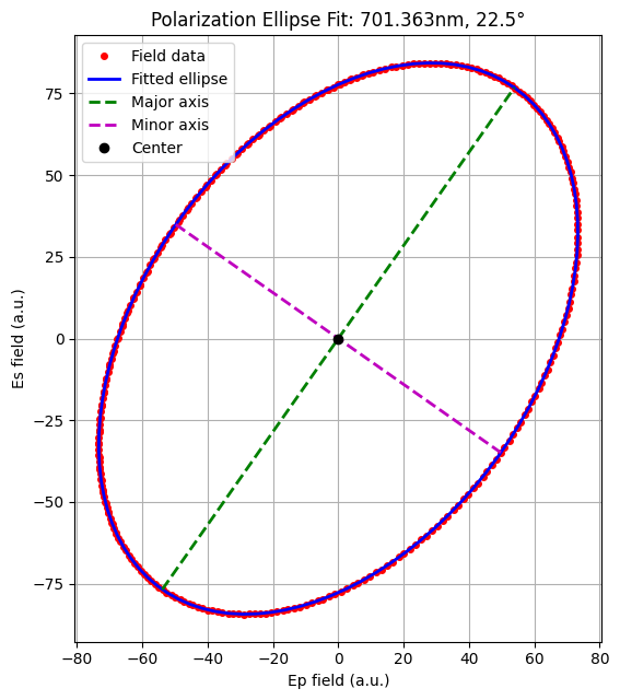
Ellipse parameters:
Center:                     (-4.45079e-05, -4.47118e-06)
Major axis a:               93.7789
Minor axis b:               60.7559
Eccentricity:               0.761756
Ellipse Orientation Angle:  54.944°
Ellipticity angle:          32.9377°
We can now repeat the process for the entire batch by sweeping through all incident angles and wavelengths:
# ---------------------
# Analyze entire batch
# ---------------------

ellipticity_by_angle = {}

for angle_deg in angle_sweeps:
    ellipticity_by_angle[angle_deg] = []

    for wl_um in wsweeps_by_angle[angle_deg]:

        # Get Ep and Es directly from batch results
        Ep, Es, t_ps = get_ep_es_from_batch(
            batch_results=batch_results,
            angle_deg=angle_deg,
            wl_um=wl_um,
            monitor_name="(0, 0) CAVITY-fieldtimemonitor",
            x0=0,
            y0=0,
            z0=0.13186,
            t_start_ps=0.9,
            n_samples=300,
        )

        # Fit ellipse and extract ellipticity angle
        ellipse_results = fit_ep_es_ellipse(Ep, Es)
        ellipticity_angle = ellipse_results["ellipticity_angle"]

        # Store result
        ellipticity_by_angle[angle_deg].append(ellipticity_angle)
Consider the ellipticity angles for all simulations with 22.5° incidence:
# ---------------------
# Table for 22.5°
# ---------------------

from IPython.display import HTML

angle_to_show = 22.5

table_22_5 = pd.DataFrame({
    "Wavelength (nm)": wsweeps_by_angle[angle_to_show] * 1e3,
    "Ellipticity Angle (°)": ellipticity_by_angle[angle_to_show],
})

table_22_5["Wavelength (nm)"] = table_22_5["Wavelength (nm)"].round(3)
table_22_5["Ellipticity Angle (°)"] = table_22_5["Ellipticity Angle (°)"].round(4)

HTML(table_22_5.to_html(index=False))
| Wavelength (nm) | Ellipticity Angle (°) |
|---|---|
| 660.000 | 44.1843 |
| 670.000 | 44.2299 |
| 680.000 | 44.1460 |
| 690.000 | 42.7783 |
| 699.863 | 35.1142 |
| 701.363 | 32.9377 |
| 703.013 | 31.4801 |
| 703.463 | 31.3844 |
| 703.863 | 31.4106 |
| 704.713 | 31.7049 |
| 706.363 | 33.0375 |
| 707.863 | 34.3548 |
| 710.000 | 35.9037 |
| 720.000 | 39.2721 |
| 730.000 | 40.4894 |
| 740.000 | 41.2036 |
This reveals an interesting correlation between the polarization state and the cavity resonance. The separate simulations mentioned earlier reveal that the resonant wavelength for light incident at 22.5° is ~703 nm. Therefore, the wavelength with the smallest ellipticity angle, corresponding to the least circular polarization, occurs in the same wavelength region as the cavity resonance. This supports the interpretation that near resonance, repeated reflections inside the cavity allow differences between the s- and p-polarized components to accumulate.
All the results can be compiled into the 2D contour plot below, which displays the ellipticity angle as a function of wavelength and incident angle.
# ------------------------
# Contour plot all points
# ------------------------

# Flatten Data into 1D Arrays
all_wavelengths_nm = []
all_angles_deg = []
all_ellipticities = []

for angle_deg in angle_sweeps:
    wl_nm = wsweeps_by_angle[angle_deg] * 1e3
    ell = ellipticity_by_angle[angle_deg]

    all_wavelengths_nm.extend(wl_nm)
    all_angles_deg.extend([angle_deg] * len(wl_nm))
    all_ellipticities.extend(ell)

all_wavelengths_nm = np.array(all_wavelengths_nm)
all_angles_deg = np.array(all_angles_deg)
all_ellipticities = np.array(all_ellipticities)

# Plot
fig, ax = plt.subplots(figsize=(8.5, 8))

levels = np.linspace(
    np.nanmin(all_ellipticities),
    np.nanmax(all_ellipticities),
    20
)

cont = ax.tricontourf(
    all_wavelengths_nm,
    all_angles_deg,
    all_ellipticities,
    levels=levels,
    cmap="coolwarm"
)

ax.tricontour(
    all_wavelengths_nm,
    all_angles_deg,
    all_ellipticities,
    levels=levels,
    colors="k",
    linewidths=0.8,
    alpha=0.5
)

cbar = fig.colorbar(cont, ax=ax)
cbar.set_label("Ellipticity Angle (°)")

ax.set_xlabel("Wavelength (nm)")
ax.set_ylabel("Incident Angle (°)")
ax.set_title("Ellipticity Angle as a Function of Wavelength and Incident Angle")

plt.tight_layout()
plt.show()
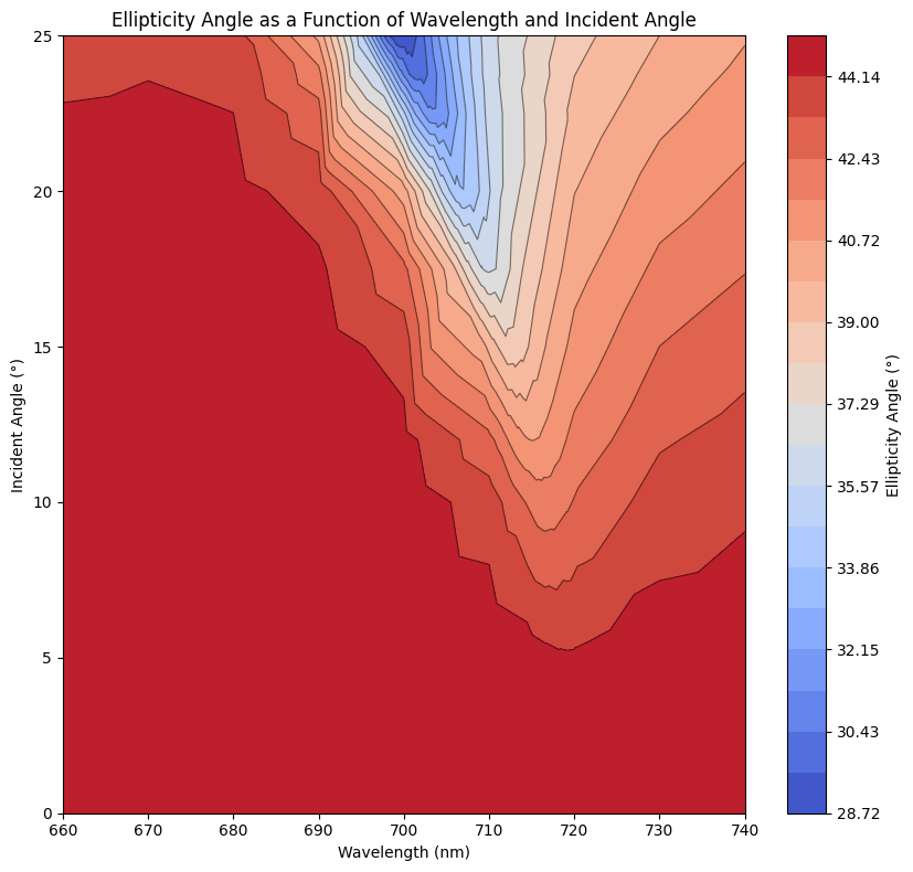
As expected, the polarization is least circular near the cavity resonance at all angles. This plot shows that the resonant wavelength decreases as incident angle increases, a trend expected from this equation for the angular dependence of the cavity resonance energy:
$E_{cav}(\theta)=\frac{E_{cav}(0)}{\sqrt{1-(\frac{\sin(\theta)}{n_{eff}})^2}}$
Additionally, the plot shows that as the incident angle increases, the cavity preserves circular polarization less effectively. This is expected because the Fresnel reflection coefficients for s- and p-polarized light differ more strongly at larger angles.
The final plot below shows ellipticity angle as a function of wavelength for a few selected incident angles. The angles of 10° and 17.5° were chosen since the cavity resonance energy at these angles matches the exciton energy in the experimental setup. As shown, at an incident angle of 10° and 17.5°, the ellipticity angle remains larger than ~42° and ~36° respectively.
# ---------------------------
# Plot a few selected slices:
# ---------------------------
angles_to_plot = [0, 10, 17.5]

fig, ax = plt.subplots(figsize=(8.5, 6.5))

for angle_deg in angles_to_plot:
    wl_nm = wsweeps_by_angle[angle_deg] * 1e3
    ell = ellipticity_by_angle[angle_deg]

    ax.plot(
        wl_nm,
        ell,
        linewidth=2,
        label=f"{angle_deg:g} Degrees"
    )

ax.set_xlabel("Wavelength (nm)")
ax.set_ylabel("Ellipticity Angle (°)")
ax.set_title("Ellipticity Angle vs. Wavelength for Selected Incidence Angles")
ax.grid(True)
ax.legend()

plt.tight_layout()
plt.show()
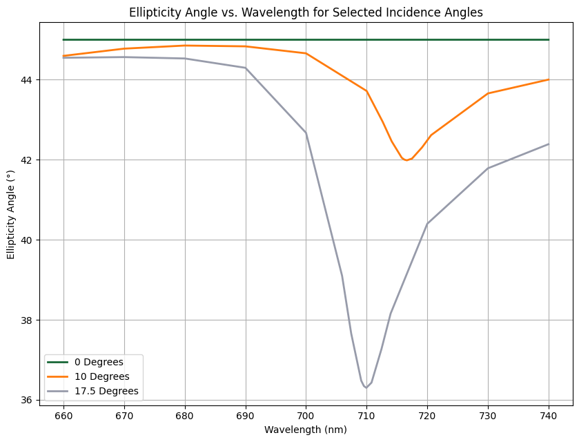
The initial goal of this simulation work was to determine whether light near cavity resonance remains sufficiently circularly polarized for valley-selective coupling. This work quantifies the degree of circular polarization for resonating light at various incident angles and wavelengths. This demonstrates that at small angles, circularity is largely maintained, consistent with the viability of valley-selective coupling.
Acknowledgments
This research was primarily supported as part of the Center for Molecular Quantum Transduction, an Energy Frontier Research Center funded by the U.S. Department of Energy (DOE), Office of Science, Basic Energy Sciences (BES), under Award No. DE-SC0021314.


 TERMS & CONDITIONS


 How the process works:
 Try this real URL to see an example: