





Authors: Azka Maula Iskandar Muda & Uğur Teğin, Koç University
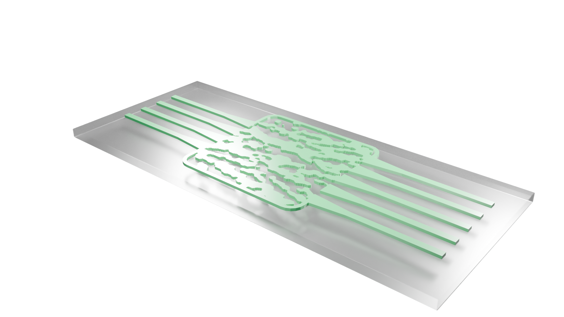
Electromagnetic optimization is expensive when the full-wave solver is included in every training step. We avoid this by first representing the optical device as a passive 5 × 4 complex matrix. The matrix is trained together with a 5 × 3 electronic readout to classify the powers measured at five output ports.
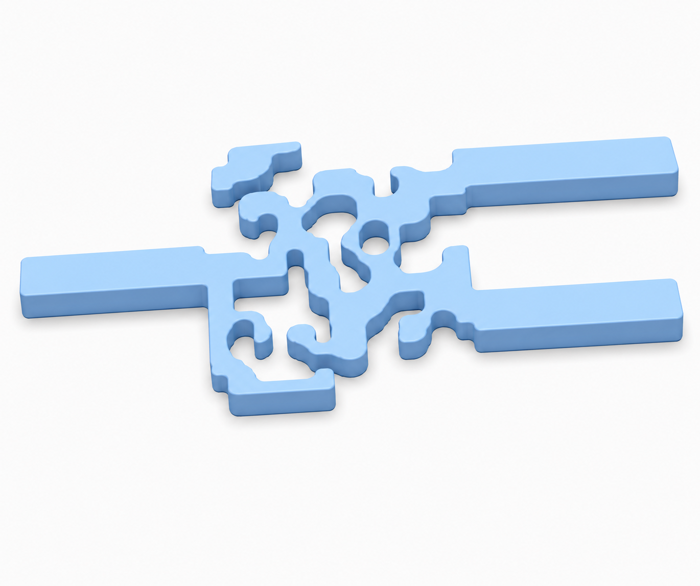
Once training is complete, the matrix is fixed and transferred to a 4-input, 5-output silicon device. Tidy3D then optimizes only the electromagnetic response, matching the complex transmission matrix while suppressing reflection and penalizing features below 200 nm.
This two-stage procedure follows our surrogate scattering-matrix workflow.
What this notebook demonstrates:
This notebook separates classifier training from electromagnetic device optimization. We first train a passive optical transformation and an electronic readout on a balanced three-class dataset. Each sample is represented by four coherent input fields, and classification uses the powers detected at five output ports.
We then fix the trained optical matrix and use Tidy3D to inverse-design a four-input, five-output silicon photonic device. The objective matches the complete complex transmission response, suppresses input reflection, and discourages solid or void features smaller than 200 nm. Finally, we evaluate how closely the simulated device reproduces the trained classifier.
Setup
The next cells install the package versions used in this example and import the tools for dataset generation, target training, visualization, and electromagnetic simulation. They also define the random seed, physical parameters, optimization schedule, and the single progress cache at output/classifier/progress.npz.
Cost estimation and cloud execution are separate operations. Their flags are False by default, so running the notebook initially performs only local calculations and device checks.
%pip install --quiet --upgrade \
    "numpy==2.4.4" "scipy==1.17.0" "matplotlib==3.10.9" \
    "scikit-learn==1.8.0" "jax==0.10.0" "optax==0.2.8" \
    "autograd==1.8.0" "gdstk==1.0.0" "tidy3d[design,extras]==2.12.0"
from __future__ import annotations

import io
from dataclasses import dataclass
from pathlib import Path

import autograd
import autograd.numpy as anp
import gdstk
import jax
import jax.numpy as jnp
import matplotlib.pyplot as plt
import numpy as np
import optax
import tidy3d as td
import tidy3d.plugins.invdes as tdi
from autograd.tracer import getval
from matplotlib_inline.backend_inline import set_matplotlib_formats
from sklearn.linear_model import LogisticRegression
from sklearn.metrics import ConfusionMatrixDisplay, confusion_matrix, log_loss
from sklearn.model_selection import train_test_split
from tidy3d import web
from tidy3d.plugins.autograd.functions import threshold
from tidy3d.plugins.autograd.invdes import make_conic_filter, smoothed_projection
from tidy3d.plugins.smatrix import ModalComponentModeler, Port
from tidy3d.plugins.smatrix.run import compose_modeler_data_from_batch_data

jax.config.update("jax_enable_x64", True)
td.config.logging.level = "ERROR"
set_matplotlib_formats("png")

DATA_SEED = 7
TRAINING_SEEDS = (7, 17, 23, 31, 47)
N_SAMPLES = 6000
N_INPUTS = 4
N_OUTPUTS = 5
N_CLASSES = 3
SEARCH_STEPS = 5000
TRAINING_STEPS = 20000
TRAINING_BATCH_SIZE = 512
ROBUST_TRAINING_LEVELS = jnp.asarray((0.05, 0.08, 0.12, 0.15))
ROBUST_TRIALS = 1000
MINIMUM_INSERTION_LOSS_DB = 3.0
MAXIMUM_TRANSMITTED_POWER = 10 ** (-MINIMUM_INSERTION_LOSS_DB / 10)
MINIMUM_OUTPUT_ROW_POWER = 0.14
OUTPUT_UTILIZATION_PENALTY_WEIGHT = 10.0

ESTIMATE_COST = True
COST_APPROVED = True
RUN_CLOUD = True
REALIZATION_UPDATES = 50
OPTIMIZATION_CREDIT_LIMIT = 25.0
RUN_SINGLE_SAMPLE_FIELD = True
SINGLE_SAMPLE_INDEX = 0

OUTPUT_DIR = Path("output") / "classifier"
OUTPUT_DIR.mkdir(parents=True, exist_ok=True)
PROGRESS_PATH = OUTPUT_DIR / "progress.npz"

if RUN_CLOUD and not (ESTIMATE_COST and COST_APPROVED):
    raise ValueError("RUN_CLOUD requires a fresh estimate and explicit cost approval.")
Photonic Classifier Concept
A sample begins with two normalized coordinates, $x$ and $y$. We form four complementary features,
$$ \mathbf v=(x,\;y,\;1-x,\;1-y), $$
so that each coordinate and its distance from the opposite boundary enter the optical system. Feature $v_j$ controls both the power and phase of one coherent input:
$$ a_j=\sqrt{v_j}\,e^{-i2\pi v_j}. $$
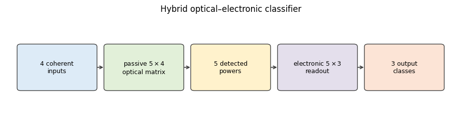
The four fields interfere inside a passive optical transformation $\mathbf T\in\mathbb C^{5\times4}$. Its five output fields are converted to detector powers,
$$ \mathbf p=\left|\mathbf a\mathbf T^{\mathsf T}\right|^2. $$
Although the optical transformation is linear in the complex fields, square-law detection makes the measured powers nonlinear functions of the original coordinates. A real-valued electronic readout then maps the five powers to three logits:
$$ \boldsymbol\ell=\mathbf p\mathbf W+\mathbf b, \qquad \mathbf W\in\mathbb R^{5\times3}. $$
The predicted class is the index of the largest logit.
from matplotlib.patches import FancyBboxPatch

fig, ax = plt.subplots(figsize=(9.2, 2.4), constrained_layout=True)
ax.set_xlim(-0.6, 4.6)
ax.set_ylim(-0.8, 0.8)
ax.axis("off")

blocks = [
    (0, "4 coherent\ninputs", "#DDEBF7"),
    (1, "passive $5\\times4$\noptical matrix", "#E2F0D9"),
    (2, "5 detected\npowers", "#FFF2CC"),
    (3, "electronic $5\\times3$\nreadout", "#E4DFEC"),
    (4, "3 output\nclasses", "#FCE4D6"),
]
for x, label, color in blocks:
    patch = FancyBboxPatch(
        (x - 0.42, -0.32),
        0.84,
        0.64,
        boxstyle="round,pad=0.04",
        facecolor=color,
        edgecolor="0.25",
    )
    ax.add_patch(patch)
    ax.text(x, 0, label, ha="center", va="center", fontsize=9)
for left, right in zip(range(4), range(1, 5)):
    ax.annotate(
        "",
        xy=(right - 0.45, 0),
        xytext=(left + 0.45, 0),
        arrowprops={"arrowstyle": "->", "lw": 1.3, "color": "0.25"},
    )
ax.set_title("Hybrid optical–electronic classifier")
plt.show()
Generate and Encode the Dataset
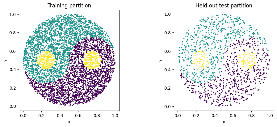
We generate 6,000 balanced samples with a fixed random seed and make a stratified 80/20 split before fitting the model. The next cell visualizes the three regions and converts every point into the four coherent input amplitudes used by the classifier.
def make_dataset(count=N_SAMPLES, seed=DATA_SEED):
    rng = np.random.default_rng(seed)
    samples, labels = [], []
    while len(samples) < count:
        requested_class = int(rng.integers(0, N_CLASSES))
        x, y = rng.random(2)
        if (x - 0.5) ** 2 + (y - 0.5) ** 2 > 0.25:
            continue
        right = np.hypot(x - 0.75, y - 0.5)
        left = np.hypot(x - 0.25, y - 0.5)
        label = (
            2
            if min(left, right) < 0.1
            else int(
                (right <= 0.1)
                or (left > 0.1 and left <= 0.25)
                or (y > 0.5 and right > 0.25)
            )
        )
        if label == requested_class:
            samples.append((x, y, 1 - x, 1 - y))
            labels.append(label)
    return np.asarray(samples), np.asarray(labels, dtype=np.int32)


def encode(values):
    values = np.asarray(values)
    return np.sqrt(values) * np.exp(-2j * np.pi * values)


raw_features, labels = make_dataset()
all_indices = np.arange(len(labels))
train_indices, test_indices = train_test_split(
    all_indices,
    test_size=0.20,
    random_state=DATA_SEED,
    stratify=labels,
)
train_x = encode(raw_features[train_indices])
test_x = encode(raw_features[test_indices])
train_y = labels[train_indices]
test_y = labels[test_indices]

fig, axes = plt.subplots(1, 2, figsize=(10, 4), constrained_layout=True)
for axis, indices, title in (
    (axes[0], train_indices, "Training partition"),
    (axes[1], test_indices, "Held-out test partition"),
):
    axis.scatter(
        raw_features[indices, 0],
        raw_features[indices, 1],
        c=labels[indices],
        cmap="viridis",
        s=7,
        linewidths=0,
    )
    axis.set(title=title, xlabel="x", ylabel="y", aspect="equal")
print(f"train={len(train_indices):,}, test={len(test_indices):,}")
train=4,800, test=1,200
Train the Optical Target
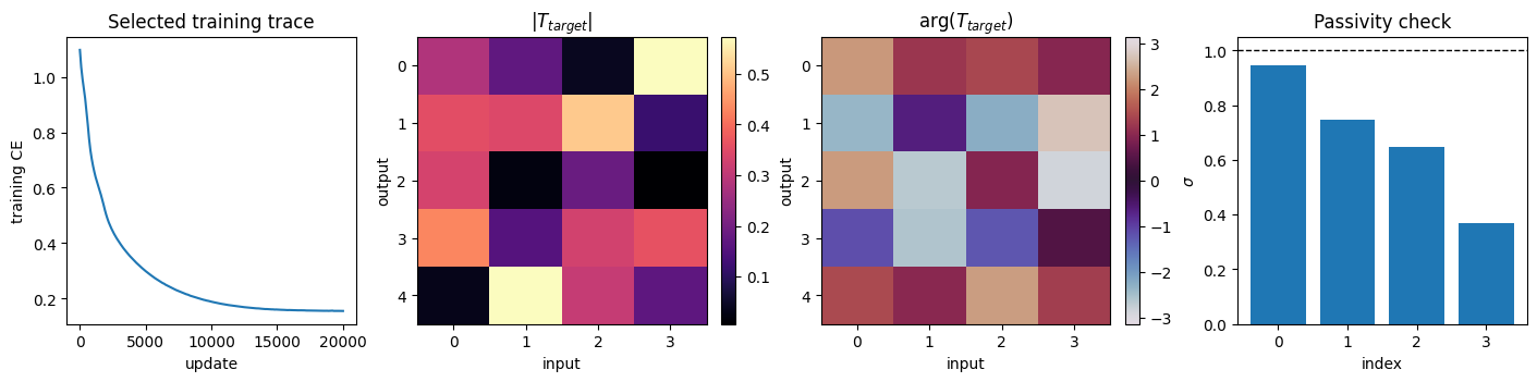
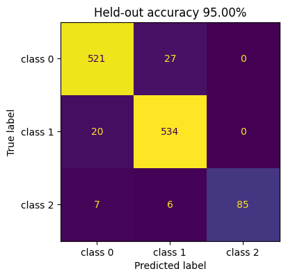
We constrain the largest singular value of the 5 × 4 target to at most one and require at least 3 dB insertion loss for every input column. Five deterministic starts are screened on training quantities, and the selected initialization is trained for 20,000 updates.
Rows with total target power below 0.14 receive a penalty so every detector contributes to the readout. The held-out partition is evaluated only after model selection.
def constrain_transmission(matrix):
    column_power = jnp.sum(jnp.abs(matrix) ** 2, axis=0)
    column_scale = jnp.sqrt(
        jnp.minimum(
            1.0,
            MAXIMUM_TRANSMITTED_POWER / jnp.maximum(column_power, 1e-15),
        )
    )
    matrix = matrix * column_scale[None, :]
    largest = jnp.linalg.svd(matrix, compute_uv=False)[0]
    return matrix / jnp.maximum(largest, 1.0)


def passive_matrix(parameters):
    raw = parameters["real"] + 1j * parameters["imag"]
    return constrain_transmission(raw)


def target_logits(parameters, fields, transmission=None):
    matrix = passive_matrix(parameters) if transmission is None else transmission
    powers = jnp.abs(jnp.asarray(fields) @ matrix.T) ** 2
    return powers @ parameters["weight"] + parameters["bias"]


def initialize_target(seed):
    keys = jax.random.split(jax.random.PRNGKey(seed), 3)
    return {
        "real": 0.1 * jax.random.normal(keys[0], (N_OUTPUTS, N_INPUTS)),
        "imag": 0.1 * jax.random.normal(keys[1], (N_OUTPUTS, N_INPUTS)),
        "weight": 0.05 * jax.random.normal(keys[2], (N_OUTPUTS, N_CLASSES)),
        "bias": jnp.zeros(N_CLASSES),
    }


def train_target(seed, steps):
    parameters = initialize_target(seed)
    optimizer = optax.adam(1e-3)
    state = optimizer.init(parameters)
    x = jnp.asarray(train_x)
    y = jnp.asarray(train_y)

    @jax.jit
    def step(
        candidate,
        optimizer_state,
        batch_x,
        batch_y,
        key,
        robust_fraction,
    ):
        def objective(trial):
            matrix = passive_matrix(trial)
            nominal = optax.softmax_cross_entropy_with_integer_labels(
                target_logits(trial, batch_x, matrix), batch_y
            ).mean()
            noise = jax.random.normal(
                key, (len(ROBUST_TRAINING_LEVELS), N_OUTPUTS, N_INPUTS)
            ) + 1j * jax.random.normal(
                jax.random.fold_in(key, 1),
                (len(ROBUST_TRAINING_LEVELS), N_OUTPUTS, N_INPUTS),
            )
            noise /= jnp.linalg.norm(noise, axis=(1, 2), keepdims=True)
            perturbed = (
                matrix[None]
                + ROBUST_TRAINING_LEVELS[:, None, None]
                * jnp.linalg.norm(matrix)
                * noise
            )
            perturbed = jax.vmap(constrain_transmission)(perturbed)
            robust = jax.vmap(
                lambda response: optax.softmax_cross_entropy_with_integer_labels(
                    target_logits(trial, batch_x, response), batch_y
                ).mean()
            )(perturbed).mean()
            row_power = jnp.sum(jnp.abs(matrix) ** 2, axis=1)
            utilization = jnp.mean(jax.nn.relu(MINIMUM_OUTPUT_ROW_POWER - row_power))
            return (
                (1.0 - robust_fraction) * nominal
                + robust_fraction * robust
                + OUTPUT_UTILIZATION_PENALTY_WEIGHT * utilization
                + 1e-4 * jnp.sum(trial["weight"] ** 2)
            )

        loss, gradient = jax.value_and_grad(objective)(candidate)
        updates, optimizer_state = optimizer.update(
            gradient, optimizer_state, candidate
        )
        return (
            optax.apply_updates(candidate, updates),
            optimizer_state,
            loss,
        )

    rng = np.random.default_rng(seed)
    history = []
    for update in range(1, steps + 1):
        indices = rng.choice(len(train_x), TRAINING_BATCH_SIZE, replace=False)
        parameters, state, loss = step(
            parameters,
            state,
            x[indices],
            y[indices],
            jax.random.PRNGKey(seed + update),
            np.clip((update - 5000) / 2000, 0.0, 0.5),
        )
        if update == 1 or update % 100 == 0:
            full_loss = float(
                optax.softmax_cross_entropy_with_integer_labels(
                    target_logits(parameters, x), y
                ).mean()
            )
            matrix = passive_matrix(parameters)
            row_power = jnp.sum(jnp.abs(matrix) ** 2, axis=1)
            utilization = jnp.mean(jax.nn.relu(MINIMUM_OUTPUT_ROW_POWER - row_power))
            selection_score = float(
                full_loss + OUTPUT_UTILIZATION_PENALTY_WEIGHT * utilization
            )
            history.append((update, float(loss), full_loss, selection_score))
    return jax.tree.map(np.asarray, parameters), np.asarray(history)
target_candidates = []
for seed in TRAINING_SEEDS:
    candidate, candidate_history = train_target(seed, SEARCH_STEPS)
    target_candidates.append(
        (candidate_history[-1, 3], seed, candidate, candidate_history)
    )
    print(f"seed {seed}: selection score={candidate_history[-1, 3]:.5f}")

_, selected_seed, _, _ = min(target_candidates, key=lambda item: item[0])
target_parameters, target_history = train_target(selected_seed, TRAINING_STEPS)
target_matrix = np.asarray(passive_matrix(target_parameters))
readout_w = np.asarray(target_parameters["weight"])
readout_b = np.asarray(target_parameters["bias"])
seed 7: selection score=0.30450
seed 17: selection score=0.30399
seed 23: selection score=0.31284
seed 31: selection score=0.29921
seed 47: selection score=0.30371
def classify(fields, transmission=target_matrix):
    powers = np.abs(np.asarray(fields) @ transmission.T) ** 2
    return np.argmax(powers @ readout_w + readout_b, axis=1)


train_accuracy = np.mean(classify(train_x) == train_y)
test_prediction = classify(test_x)
test_accuracy = np.mean(test_prediction == test_y)
singular_values = np.linalg.svd(target_matrix, compute_uv=False)

print(f"selected seed: {selected_seed}")
print(f"training accuracy: {train_accuracy:.2%}")
print(f"held-out accuracy: {test_accuracy:.2%}")
print(f"largest singular value: {singular_values[0]:.6f}")
target_input_power = np.sum(np.abs(target_matrix) ** 2, axis=0)
target_insertion_loss_db = -10 * np.log10(np.maximum(target_input_power, 1e-15))
print(
    "target insertion loss per input (dB):",
    np.round(target_insertion_loss_db, 4),
)
target_output_power = np.sum(np.abs(target_matrix) ** 2, axis=1)
print(
    "target power per output:",
    np.round(target_output_power, 5),
)
if not np.all(target_input_power <= MAXIMUM_TRANSMITTED_POWER + 1e-10):
    raise ValueError("The trained target violates the insertion-loss constraint.")
if not np.all(target_output_power >= MINIMUM_OUTPUT_ROW_POWER - 1e-3):
    raise ValueError("The trained target violates the output-power constraint.")
selected seed: 31
training accuracy: 95.83%
held-out accuracy: 95.00%
largest singular value: 0.944694
target insertion loss per input (dB): [3. 3. 3. 3.]
target power per output: [0.43828 0.51904 0.14476 0.44821 0.45446]
fig, axes = plt.subplots(1, 4, figsize=(14, 3.4), constrained_layout=True)
axes[0].plot(target_history[:, 0], target_history[:, 2])
axes[0].set(title="Selected training trace", xlabel="update", ylabel="training CE")
amplitude = axes[1].imshow(np.abs(target_matrix), cmap="magma", aspect="auto")
axes[1].set(title=r"$|T_{target}|$", xlabel="input", ylabel="output")
fig.colorbar(amplitude, ax=axes[1])
phase = axes[2].imshow(
    np.angle(target_matrix),
    cmap="twilight",
    vmin=-np.pi,
    vmax=np.pi,
    aspect="auto",
)
axes[2].set(title=r"$\arg(T_{target})$", xlabel="input", ylabel="output")
fig.colorbar(phase, ax=axes[2])
axes[3].bar(np.arange(len(singular_values)), singular_values)
axes[3].axhline(1, color="black", linestyle="--", linewidth=1)
axes[3].set(title="Passivity check", xlabel="index", ylabel=r"$\sigma$")

fig, ax = plt.subplots(figsize=(4, 4), constrained_layout=True)
ConfusionMatrixDisplay(
    confusion_matrix(test_y, test_prediction),
    display_labels=("class 0", "class 1", "class 2"),
).plot(ax=ax, colorbar=False)
ax.set_title(f"Held-out accuracy {test_accuracy:.2%}")
Text(0.5, 1.0, 'Held-out accuracy 95.00%')
Evaluate Matrix Perturbations
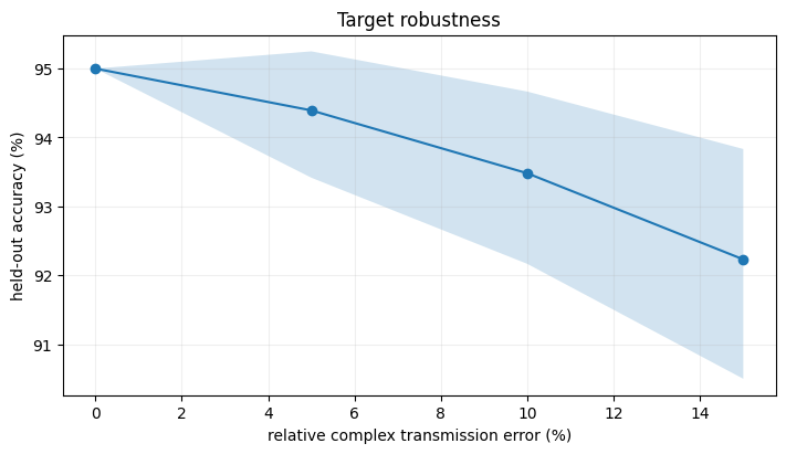
We apply 1,000 reproducible complex perturbations at each tested error level. Every perturbed matrix keeps spectral norm at most one and at least 3 dB insertion loss per input. This calculation measures target sensitivity without an electromagnetic solve.
ROBUST_LEVELS = np.asarray((0.0, 0.05, 0.10, 0.15))
rng = np.random.default_rng(DATA_SEED + 10_000)
robust_accuracy = np.empty((len(ROBUST_LEVELS), ROBUST_TRIALS))
target_norm = np.linalg.norm(target_matrix)
for level_index, level in enumerate(ROBUST_LEVELS):
    for trial in range(ROBUST_TRIALS):
        if level == 0:
            perturbed = target_matrix
        else:
            noise = rng.standard_normal(target_matrix.shape) + 1j * rng.standard_normal(
                target_matrix.shape
            )
            noise *= level * target_norm / np.linalg.norm(noise)
            perturbed = target_matrix + noise
            column_power = np.sum(np.abs(perturbed) ** 2, axis=0)
            perturbed *= np.sqrt(
                np.minimum(
                    1.0,
                    MAXIMUM_TRANSMITTED_POWER / np.maximum(column_power, 1e-15),
                )
            )[None, :]
            perturbed /= max(np.linalg.svd(perturbed, compute_uv=False)[0], 1.0)
        robust_accuracy[level_index, trial] = np.mean(
            classify(test_x, perturbed) == test_y
        )

robust_mean = robust_accuracy.mean(axis=1)
robust_p5 = np.percentile(robust_accuracy, 5, axis=1)
robust_p95 = np.percentile(robust_accuracy, 95, axis=1)
fig, ax = plt.subplots(figsize=(7, 4), constrained_layout=True)
ax.plot(100 * ROBUST_LEVELS, 100 * robust_mean, marker="o")
ax.fill_between(100 * ROBUST_LEVELS, 100 * robust_p5, 100 * robust_p95, alpha=0.2)
ax.set(
    title="Target robustness",
    xlabel="relative complex transmission error (%)",
    ylabel="held-out accuracy (%)",
)
ax.grid(alpha=0.2)
Set Up the Silicon Photonic Device
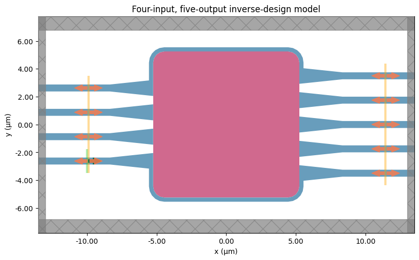
The physical model uses a 10.5 µm square design region with four inputs, five outputs, 1.75 µm port pitch and modal windows, zero taper intrusion, and 300 nm rounded rail bridges.
We use silica index 1.4447002763 and variational quasi-TE indices for the 150 nm and 220 nm silicon states. Filtering acts on the full square parameter field, and a higher-priority silica structure removes the rounded corners afterward. The following cells calibrate the effective indices, construct the geometry, inspect the modes, and validate all four source simulations before upload.
WAVELENGTH_UM = 1.55
DEVICE_EDGE_UM = 2.1 * max(N_INPUTS, N_OUTPUTS)
CORE_THICKNESS_UM = 0.22
WAVEGUIDE_WIDTH_UM = 0.50
PORT_PITCH_UM = 1.75
TAPER_LENGTH_UM = 3.10
TAPER_MOUTH_UM = 1.15
CORNER_RADIUS_UM = 0.80
RAIL_THICKNESS_UM = 0.30
PML_EXTENSION_UM = 2.0
MODE_WINDOW_UM = 1.75

PIXEL_SIZE_UM = 0.050
FILTER_RADIUS_UM = 0.200
MINIMUM_FEATURE_UM = 0.200
PROJECTION_BETA_INITIAL = 50.0
PROJECTION_BETA_FINAL = 50.0
PROJECTION_ETA = 0.5
FABRICATION_WEIGHT_MAX = 0.8
FABRICATION_START_UPDATE = 6
FABRICATION_FULL_UPDATE = 15
FABRICATION_BETA = 100.0
FABRICATION_ETA0 = 0.5
FABRICATION_DELTA_ETA = 0.01

ADAM_BETA1 = 0.9
ADAM_BETA2 = 0.999
ADAM_EPSILON = 1e-8
ADAM_STEP_MAX_ABS = 0.02
FREQUENCY_HZ = td.C_0 / WAVELENGTH_UM
N_CLAD = 1.4447002763
N_EFF_150_VALIDATED = 2.4528810767646334
N_EFF_220_VALIDATED = 2.7956415856033523
td.config.simulation.use_local_subpixel = True


@dataclass(frozen=True)
class EffectiveIndexCalibration:
    n_eff_150: float
    n_eff_220: float
    n_background: float

    @property
    def eps_design(self):
        return self.n_eff_150**2, self.n_eff_220**2


def calibrate_effective_indices() -> EffectiveIndexCalibration:
    return EffectiveIndexCalibration(
        n_eff_150=N_EFF_150_VALIDATED,
        n_eff_220=N_EFF_220_VALIDATED,
        n_background=N_CLAD,
    )
class SmoothedFilterProject(tdi.FilterProject):
    def evaluate(self, spatial_data, design_region_dl, symmetry=None):
        if symmetry is not None:
            raise ValueError("Smoothed projection requires no design symmetry.")
        singleton_z = spatial_data.ndim == 3 and spatial_data.shape[-1] == 1
        plane = spatial_data[..., 0] if singleton_z else spatial_data
        plane = anp.clip(plane, 0.0, 1.0)
        filtered = make_conic_filter(
            radius=self.radius, dl=design_region_dl, padding="edge"
        )(plane)
        projected = smoothed_projection(
            filtered,
            beta=self.beta,
            eta=self.eta,
            scaling_factor=1.0,
        )
        if self.strict_binarize:
            projected = threshold(projected)
        projected = anp.clip(projected, 0.0, 1.0)
        return projected[..., None] if singleton_z else projected


def fabrication_penalty():
    return tdi.ErosionDilationPenalty(
        weight=1.0,
        length_scale=MINIMUM_FEATURE_UM,
        beta=FABRICATION_BETA,
        eta0=FABRICATION_ETA0,
        delta_eta=FABRICATION_DELTA_ETA,
    )


def design_region(calibration, projection_beta=None):
    edge = DEVICE_EDGE_UM
    if projection_beta is None:
        projection_beta = PROJECTION_BETA_INITIAL
    return tdi.TopologyDesignRegion(
        size=(edge, edge, CORE_THICKNESS_UM),
        center=(0, 0, 0),
        eps_bounds=calibration.eps_design,
        transformations=(
            SmoothedFilterProject(
                radius=FILTER_RADIUS_UM,
                beta=projection_beta,
                eta=PROJECTION_ETA,
            ),
        ),
        penalties=(),
        initialization_spec=tdi.UniformInitializationSpec(value=0.5),
        pixel_size=PIXEL_SIZE_UM,
        uniform=(False, False, True),
        priority=0,
    )


def design_active_mask():
    edge = DEVICE_EDGE_UM
    count = round(edge / PIXEL_SIZE_UM)
    coordinates = (np.arange(count) + 0.5) * PIXEL_SIZE_UM - edge / 2
    xx, yy = np.meshgrid(coordinates, coordinates, indexing="ij")
    inner = edge / 2 - CORNER_RADIUS_UM
    dx = np.maximum(np.abs(xx) - inner, 0.0)
    dy = np.maximum(np.abs(yy) - inner, 0.0)
    mask = dx**2 + dy**2 <= CORNER_RADIUS_UM**2
    return mask[..., None]
def port_positions(count: int, pitch: float = PORT_PITCH_UM):
    return (np.arange(count) - (count - 1) / 2) * pitch


def vertices(xs, widths, y):
    xs, widths = np.asarray(xs), np.asarray(widths)
    lower = np.c_[xs, y - widths / 2]
    upper = np.c_[xs[::-1], (y + widths / 2)[::-1]]
    return np.r_[lower, upper]


def rounded_box(length, width, radius, layer):
    polygon = gdstk.rectangle(
        (-length / 2, -width / 2), (length / 2, width / 2), layer=layer
    )
    polygon.fillet(radius)
    return polygon


def device_coordinates():
    half = DEVICE_EDGE_UM / 2
    left = -half - TAPER_LENGTH_UM - 4.65
    right = half + TAPER_LENGTH_UM + 4.65
    return {
        "half": half,
        "domain_x": (left, right),
        "domain_y": (-half - 1.55, half + 1.55),
        "source_x": -half - TAPER_LENGTH_UM - 2.325,
        "input_monitor_x": -half - TAPER_LENGTH_UM - 1.55,
        "output_monitor_x": right - 1.55,
    }


def fixed_device_polygons():
    layer, polygons = 3, []
    coordinates = device_coordinates()
    half = coordinates["half"]
    domain_x = coordinates["domain_x"]
    taper_left = -half - TAPER_LENGTH_UM
    taper_right = half + TAPER_LENGTH_UM
    input_y = port_positions(N_INPUTS)
    output_y = port_positions(N_OUTPUTS)
    for y in input_y:
        polygons.extend(
            [
                gdstk.rectangle(
                    (
                        domain_x[0] - PML_EXTENSION_UM,
                        y - WAVEGUIDE_WIDTH_UM / 2,
                    ),
                    (taper_left, y + WAVEGUIDE_WIDTH_UM / 2),
                    layer=layer,
                ),
                gdstk.Polygon(
                    vertices(
                        np.linspace(taper_left, -half, 101),
                        np.linspace(
                            WAVEGUIDE_WIDTH_UM,
                            TAPER_MOUTH_UM,
                            101,
                        ),
                        y,
                    ),
                    layer=layer,
                ),
            ]
        )
    for y in output_y:
        polygons.extend(
            [
                gdstk.Polygon(
                    vertices(
                        np.linspace(half, taper_right, 101),
                        np.linspace(
                            TAPER_MOUTH_UM,
                            WAVEGUIDE_WIDTH_UM,
                            101,
                        ),
                        y,
                    ),
                    layer=layer,
                ),
                gdstk.rectangle(
                    (taper_right, y - WAVEGUIDE_WIDTH_UM / 2),
                    (
                        domain_x[1] + PML_EXTENSION_UM,
                        y + WAVEGUIDE_WIDTH_UM / 2,
                    ),
                    layer=layer,
                ),
            ]
        )
    rail = RAIL_THICKNESS_UM
    outer = rounded_box(
        2 * half + 2 * rail,
        2 * half + 2 * rail,
        CORNER_RADIUS_UM + rail,
        layer,
    )
    inner = rounded_box(
        2 * half,
        2 * half,
        CORNER_RADIUS_UM,
        layer,
    )
    ring = gdstk.boolean([outer], [inner], "not", layer=layer, precision=1e-9) or []
    mask_bound = half + 0.5
    windows = []
    for x0, x1, positions in (
        (-mask_bound, 0, input_y),
        (0, mask_bound, output_y),
    ):
        lower = positions[0] - TAPER_MOUTH_UM / 2
        upper = positions[-1] + TAPER_MOUTH_UM / 2
        windows.extend(
            [
                gdstk.rectangle((x0, -mask_bound), (x1, lower), layer=layer),
                gdstk.rectangle((x0, upper), (x1, mask_bound), layer=layer),
            ]
        )
    polygons.extend(
        gdstk.boolean(ring, windows, "and", layer=layer, precision=1e-9) or []
    )
    bridges = []
    for x0, x1, positions in (
        (-mask_bound, -half, input_y),
        (half, mask_bound, output_y),
    ):
        bridges.extend(
            [
                gdstk.rectangle(
                    (
                        x0,
                        positions[0] - TAPER_MOUTH_UM / 2 - rail,
                    ),
                    (x1, positions[0]),
                    layer=layer,
                ),
                gdstk.rectangle(
                    (x0, positions[-1]),
                    (
                        x1,
                        positions[-1] + TAPER_MOUTH_UM / 2 + rail,
                    ),
                    layer=layer,
                ),
            ]
        )
    polygons.extend(
        gdstk.boolean(ring, bridges, "and", layer=layer, precision=1e-9) or []
    )
    return gdstk.boolean(polygons, [], "or", layer=layer, precision=1e-9) or []


def corner_mask_polygons():
    edge = DEVICE_EDGE_UM
    half = edge / 2
    rectangle = gdstk.rectangle((-half, -half), (half, half), layer=4)
    rounded = rounded_box(edge, edge, CORNER_RADIUS_UM, layer=4)
    return gdstk.boolean([rectangle], [rounded], "not", layer=4, precision=1e-9) or []


def geometry_from_gds(polygons, layer):
    library = gdstk.Library()
    cell = library.new_cell(f"GEOMETRY_{layer}")
    cell.add(*polygons)
    return td.Geometry.from_gds(
        cell,
        axis=2,
        slab_bounds=(
            -CORE_THICKNESS_UM / 2,
            CORE_THICKNESS_UM / 2,
        ),
        gds_layer=layer,
        gds_dtype=0,
        reference_plane="middle",
    )
def device_base_simulation(calibration: EffectiveIndexCalibration):
    coordinates = device_coordinates()
    core = td.Medium(permittivity=calibration.n_eff_220**2)
    clad = td.Medium(permittivity=calibration.n_background**2)
    return td.Simulation(
        center=(0, 0, 0),
        size=(
            np.ptp(coordinates["domain_x"]),
            np.ptp(coordinates["domain_y"]),
            0,
        ),
        medium=clad,
        structures=[
            td.Structure(
                geometry=geometry_from_gds(fixed_device_polygons(), 3),
                medium=core,
                name="fixed_rails_tapers",
                priority=2,
            ),
            td.Structure(
                geometry=geometry_from_gds(corner_mask_polygons(), 4),
                medium=clad,
                name="rounded_corner_mask",
                priority=1,
            ),
        ],
        sources=[],
        monitors=[],
        run_time=15e-12,
        shutoff=1e-4,
        grid_spec=td.GridSpec.auto(wavelength=WAVELENGTH_UM, min_steps_per_wvl=13),
        boundary_spec=td.BoundarySpec(
            x=td.Boundary.pml(),
            y=td.Boundary.pml(),
            z=td.Boundary.periodic(),
        ),
        subpixel=True,
    )


@dataclass(frozen=True)
class ModalSimulationFactory:
    calibration: EffectiveIndexCalibration
    region: tdi.TopologyDesignRegion
    simulation: td.Simulation
    ports: tuple[Port, ...]
    input_names: tuple[str, ...]
    output_names: tuple[str, ...]

    def modeler(
        self,
        parameters,
        input_names: tuple[str, ...] | None = None,
    ) -> ModalComponentModeler:
        structure = self.region.to_structure(parameters)
        simulation = self.simulation.updated_copy(
            structures=(*self.simulation.structures, structure)
        )
        selected_inputs = self.input_names if input_names is None else input_names
        return ModalComponentModeler(
            name="classifier_modal",
            simulation=simulation,
            ports=self.ports,
            freqs=(FREQUENCY_HZ,),
            run_only=tuple((name, 0) for name in selected_inputs),
        )


def build_modal_factory(
    calibration: EffectiveIndexCalibration,
    projection_beta=None,
) -> ModalSimulationFactory:
    coordinates = device_coordinates()
    mode_spec = td.ModeSpec(
        num_modes=1,
        target_neff=calibration.n_eff_220,
    )
    input_names = tuple(f"input_{index:02d}" for index in range(N_INPUTS))
    output_names = tuple(f"output_{index:02d}" for index in range(N_OUTPUTS))
    inputs = tuple(
        Port(
            center=(coordinates["input_monitor_x"], float(y), 0),
            size=(0, MODE_WINDOW_UM, td.inf),
            name=name,
            direction="+",
            mode_spec=mode_spec,
        )
        for name, y in zip(input_names, port_positions(N_INPUTS))
    )
    outputs = tuple(
        Port(
            center=(coordinates["output_monitor_x"], float(y), 0),
            size=(0, MODE_WINDOW_UM, td.inf),
            name=name,
            direction="-",
            mode_spec=mode_spec,
        )
        for name, y in zip(output_names, port_positions(N_OUTPUTS))
    )
    return ModalSimulationFactory(
        calibration=calibration,
        region=design_region(calibration, projection_beta=projection_beta),
        simulation=device_base_simulation(calibration),
        ports=inputs + outputs,
        input_names=input_names,
        output_names=output_names,
    )
calibration = calibrate_effective_indices()
factory = build_modal_factory(calibration)
initial_parameters = factory.region.initial_parameters
modeler = factory.modeler(initial_parameters)

if target_matrix.shape != (N_OUTPUTS, N_INPUTS) or len(modeler.sim_dict) != N_INPUTS:
    raise ValueError("Target dimensions or source simulation count are incorrect.")
for simulation in modeler.sim_dict.values():
    simulation.validate_pre_upload()

print(f"design edge: {DEVICE_EDGE_UM:.1f} µm")
print(f"design parameters: {initial_parameters.size:,}")
print(f"source simulations: {len(modeler.sim_dict)}")
print(
    f"n_eff(150 nm)={calibration.n_eff_150:.6f}, "
    f"n_eff(220 nm)={calibration.n_eff_220:.6f}"
)

first_simulation = next(iter(modeler.sim_dict.values()))
fig, ax = plt.subplots(figsize=(10, 5), constrained_layout=True)
first_simulation.plot(z=0, ax=ax)
ax.set_title("Four-input, five-output inverse-design model")
design edge: 10.5 µm
design parameters: 44,100
source simulations: 4
n_eff(150 nm)=2.452881, n_eff(220 nm)=2.795642
Text(0.5, 1.0, 'Four-input, five-output inverse-design model')
Define the Realization Objective
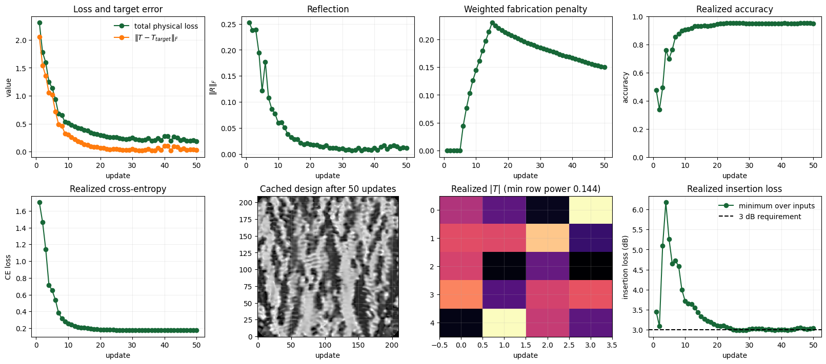
Each optimizer evaluation launches all four inputs and extracts the complete incident-normalized transmission and reflection blocks. The loss is
$$ \mathcal L= \lVert\mathbf T-\mathbf T_{\mathrm{target}}\rVert_F+ \lVert\mathbf R\rVert_F+ w_{\mathrm{fab}}\mathcal P_{\mathrm{ED}}. $$
The unsquared complex Frobenius terms respond to amplitude and phase mismatch while preserving coherent interference between inputs. The erosion–dilation term penalizes narrow silicon and void features with its scheduled weight.
We keep the trained target fixed during realization. Insertion loss and output-row power are displayed as diagnostics but do not alter the objective. The relative transmission error is calculated from the current response as $\lVert\mathbf T-\mathbf T_{\mathrm{target}}\rVert_F/\lVert\mathbf T_{\mathrm{target}}\rVert_F$.
@dataclass(frozen=True)
class ScatteringResponse:
    transmission: object
    reflection: object
    incident: object


def _numeric_value(value):
    return np.asarray(getattr(value, "_value", value))


def _smatrix_element(
    smatrix,
    port_out: str,
    port_in: str,
    frequency_hz: float,
):
    value = (
        smatrix.sel(
            port_out=port_out,
            mode_index_out=0,
            port_in=port_in,
            mode_index_in=0,
        )
        .sel(f=frequency_hz, method="nearest")
        .data
    )
    return value.item() if np.ndim(value) == 0 else anp.squeeze(value)


def response_from_batch(
    modeler,
    batch_data,
    input_names: tuple[str, ...],
    output_names: tuple[str, ...],
    frequency_hz: float,
    reflection_names: tuple[str, ...] | None = None,
) -> ScatteringResponse:
    reflection_names = input_names if reflection_names is None else reflection_names
    modeler_data = compose_modeler_data_from_batch_data(
        modeler=modeler, batch_data=batch_data
    )
    smatrix = modeler_data.smatrix()
    transmissions = []
    reflections = []
    incidents = []
    for input_name in input_names:
        port = modeler.get_port_by_name(port_name=input_name)
        task_name = modeler.get_task_name(port=port, mode_index=0)
        incident = modeler._normalization_factor(port, modeler_data.data[task_name])
        incident_value = _numeric_value(incident)
        if not np.all(np.isfinite(incident_value)) or np.any(
            np.abs(incident_value) == 0
        ):
            raise ValueError(
                f"Invalid incident amplitude for {input_name}: {incident_value}"
            )
        incidents.append(incident)
        transmissions.append(
            anp.stack(
                [
                    _smatrix_element(smatrix, output_name, input_name, frequency_hz)
                    for output_name in output_names
                ]
            )
        )
        reflections.append(
            anp.stack(
                [
                    _smatrix_element(smatrix, reflected_name, input_name, frequency_hz)
                    for reflected_name in reflection_names
                ]
            )
        )
    return ScatteringResponse(
        transmission=anp.stack(transmissions, axis=1),
        reflection=anp.stack(reflections, axis=1),
        incident=anp.stack(incidents),
    )
def run_modeler_batch(modeler, path_dir):
    from tidy3d.web import run_async

    path_dir = Path(path_dir)
    path_dir.mkdir(parents=True, exist_ok=True)
    data = {}
    items = list(modeler.sim_dict.items())
    for start in range(0, len(items), 8):
        chunk = dict(items[start : start + 8])
        batch = run_async(chunk, path_dir=path_dir, verbose=False)
        for name in chunk:
            data[name] = batch[name]
    return data


def frobenius(values):
    squared_norm = anp.sum(anp.real(values * anp.conj(values)))
    return anp.sqrt(squared_norm + 1e-24)


def fabrication_weight(update):
    if update < FABRICATION_START_UPDATE:
        return 0.0
    if update >= FABRICATION_FULL_UPDATE:
        return FABRICATION_WEIGHT_MAX
    ramp_updates = FABRICATION_FULL_UPDATE - FABRICATION_START_UPDATE + 1
    return (
        FABRICATION_WEIGHT_MAX * (update - FABRICATION_START_UPDATE + 1) / ramp_updates
    )


def learning_rate(update):
    return 0.01 * update if update <= 5 else 0.05


def projection_beta(update):
    return PROJECTION_BETA_FINAL


def realization_score(factory, target, weight, response_dir):
    penalty = fabrication_penalty()

    def score(parameters, auxiliary=None):
        modeler = factory.modeler(parameters)
        batch = run_modeler_batch(modeler, response_dir)
        response = response_from_batch(
            modeler,
            batch,
            factory.input_names,
            factory.output_names,
            FREQUENCY_HZ,
        )
        density = factory.region.material_density(parameters)
        morphology = penalty.evaluate(density, PIXEL_SIZE_UM)
        transmission_loss = frobenius(response.transmission - target)
        reflection_loss = frobenius(response.reflection)
        transmitted_power = anp.sum(
            anp.real(response.transmission * anp.conj(response.transmission)),
            axis=0,
        )
        output_row_power = anp.sum(
            anp.real(response.transmission * anp.conj(response.transmission)),
            axis=1,
        )
        total = transmission_loss + reflection_loss + weight * morphology
        if auxiliary is not None:
            auxiliary.update(
                {
                    "transmission": getval(response.transmission),
                    "reflection": getval(response.reflection),
                    "incident": getval(response.incident),
                    "transmission_loss": getval(transmission_loss),
                    "reflection_loss": getval(reflection_loss),
                    "fabrication": getval(morphology),
                    "transmitted_power": getval(transmitted_power),
                    "output_row_power": getval(output_row_power),
                }
            )
        return -total

    return score


print("learning rates 1–8:", [learning_rate(i) for i in range(1, 9)])
print("fabrication weights 1–16:", [fabrication_weight(i) for i in range(1, 17)])
print("projection beta 1–50:", [projection_beta(i) for i in range(1, 51)])
learning rates 1–8: [0.01, 0.02, 0.03, 0.04, 0.05, 0.05, 0.05, 0.05]
fabrication weights 1–16: [0.0, 0.0, 0.0, 0.0, 0.0, 0.08, 0.16, 0.24000000000000005, 0.32, 0.4, 0.4800000000000001, 0.56, 0.64, 0.72, 0.8, 0.8]
projection beta 1–50: [50.0, 50.0, 50.0, 50.0, 50.0, 50.0, 50.0, 50.0, 50.0, 50.0, 50.0, 50.0, 50.0, 50.0, 50.0, 50.0, 50.0, 50.0, 50.0, 50.0, 50.0, 50.0, 50.0, 50.0, 50.0, 50.0, 50.0, 50.0, 50.0, 50.0, 50.0, 50.0, 50.0, 50.0, 50.0, 50.0, 50.0, 50.0, 50.0, 50.0, 50.0, 50.0, 50.0, 50.0, 50.0, 50.0, 50.0, 50.0, 50.0, 50.0]
Estimate Cloud Cost
Set ESTIMATE_COST=True to upload one representative source simulation for pricing. The cell deletes the estimate-only task, scales the forward cost to all four sources, and projects one forward and one adjoint batch for each remaining update.
fresh_forward_cost = None
projected_optimization_cost = None
if ESTIMATE_COST:
    name, simulation = next(iter(modeler.sim_dict.items()))
    task_id = web.upload(
        simulation,
        task_name=f"{name}_cost_only",
        folder_name="classifier_cost",
    )
    per_source_cost = float(web.estimate_cost(task_id))
    web.delete(task_id)
    fresh_forward_cost = N_INPUTS * per_source_cost
    completed_updates = 0
    if PROGRESS_PATH.exists():
        with np.load(PROGRESS_PATH, allow_pickle=False) as saved:
            completed_updates = int(saved["update"])
    remaining_updates = REALIZATION_UPDATES - completed_updates
    projected_optimization_cost = 2 * remaining_updates * fresh_forward_cost
    print(f"four-source forward batch: {fresh_forward_cost:.6f} FlexCredits")
    print(
        f"{remaining_updates} remaining forward+adjoint updates: "
        f"{projected_optimization_cost:.6f} FlexCredits"
    )
    if projected_optimization_cost > OPTIMIZATION_CREDIT_LIMIT:
        raise ValueError("Projected optimization cost exceeds the 25-credit limit.")
else:
    print("Cost estimation is disabled.")
22:22:58 KST Created task 'input_00@0_cost_only' with resource_id
             'fdve-98585daf-b65a-45ec-bbc5-2b5891e17461' and task_type 'FDTD'.
             View task using web UI at
             'https://tidy3d.simulation.cloud/workbench?taskId=fdve-98585daf-b65
             a-45ec-bbc5-2b5891e17461'.
Task folder: 'default'.
Output()
22:23:01 KST Estimated FlexCredit cost: 0.046. This assumes the FDTD solver runs
             for the full simulation time; if early shutoff is reached, the
             billed cost can be lower. Use 'web.real_cost(task_id)' to get the
             billed FlexCredit cost after a simulation run.
22:23:03 KST Estimated FlexCredit cost: 0.046. This assumes the FDTD solver runs
             for the full simulation time; if early shutoff is reached, the
             billed cost can be lower. Use 'web.real_cost(task_id)' to get the
             billed FlexCredit cost after a simulation run.
four-source forward batch: 0.182985 FlexCredits
0 remaining forward+adjoint updates: 0.000000 FlexCredits
Run the Inverse Design
The first five Adam updates use learning rates 0.01, 0.02, 0.03, 0.04, and 0.05; later updates use 0.05. The fabrication weight is zero through update 5, rises from 0.08 at update 6 to 0.8 at update 15, and follows the configured late-stage schedule. Each saved response is the optimizer-forward evaluation produced before its update.
Set COST_APPROVED=True and RUN_CLOUD=True only after this kernel has produced a fresh estimate within the configured credit limit.
Save and Resume the Optimization
After each update, we save the current design, Adam state, scattering matrices, and optimization history to output/classifier/progress.npz. If the run is interrupted, rerunning the notebook loads this file and continues from the next update. When all 50 updates are already available, the cloud loop is skipped and the cached result is used directly in the analysis.
@dataclass(frozen=True)
class AdamState:
    m: np.ndarray
    v: np.ndarray
    t: int


HISTORY_NAMES = (
    "score_history",
    "transmission_loss_history",
    "reflection_loss_history",
    "fabrication_penalty_history",
    "fabrication_weight_history",
    "projection_beta_history",
    "gray_fraction_01_99_history",
    "gray_fraction_10_90_history",
    "realized_accuracy_history",
    "realized_ce_loss_history",
    "minimum_insertion_loss_db_history",
    "minimum_output_row_power_history",
)


def save_npz_atomic(path, **arrays):
    path.parent.mkdir(parents=True, exist_ok=True)
    buffer = io.BytesIO()
    np.savez_compressed(buffer, **arrays)
    temporary = path.with_suffix(".tmp")
    temporary.write_bytes(buffer.getvalue())
    temporary.replace(path)


def load_progress(initial, active_mask):
    empty_history = {name: [] for name in HISTORY_NAMES}
    if not PROGRESS_PATH.exists():
        zeros = np.zeros_like(initial)
        return initial, AdamState(zeros, zeros, 0), 0, empty_history

    with np.load(PROGRESS_PATH, allow_pickle=False) as saved:
        update = int(saved["update"])
        checks = (
            int(saved["n_inputs"]) == N_INPUTS,
            int(saved["n_outputs"]) == N_OUTPUTS,
            int(saved["n_classes"]) == N_CLASSES,
            int(saved["realization_updates"]) == REALIZATION_UPDATES,
            np.isclose(float(saved["pixel_um"]), PIXEL_SIZE_UM),
            np.isclose(float(saved["filter_radius_um"]), FILTER_RADIUS_UM),
            np.isclose(float(saved["minimum_feature_um"]), MINIMUM_FEATURE_UM),
            np.isclose(float(saved["n_eff_150"]), calibration.n_eff_150),
            np.isclose(float(saved["n_eff_220"]), calibration.n_eff_220),
            np.array_equal(saved["target_matrix"], target_matrix),
        )
        if not all(checks):
            raise ValueError("Progress cache does not match this classifier.")
        parameters = np.asarray(saved["parameters_after"])
        state = AdamState(
            np.asarray(saved["adam_m"]),
            np.asarray(saved["adam_v"]),
            int(saved["adam_t"]),
        )
        history = {
            name: list(np.asarray(saved[name], dtype=float)) for name in HISTORY_NAMES
        }

    if (
        parameters.shape != initial.shape
        or state.m.shape != initial.shape
        or state.v.shape != initial.shape
        or state.t != update
        or any(len(values) != update for values in history.values())
    ):
        raise ValueError("Cached Adam state does not match completed updates.")
    return (
        np.where(active_mask, parameters, 0.0),
        state,
        update,
        history,
    )


def adam_ascent(parameters, gradient, state, update, active_mask):
    gradient = np.where(active_mask, gradient, 0.0)
    t = state.t + 1
    m = ADAM_BETA1 * state.m + (1 - ADAM_BETA1) * gradient
    v = ADAM_BETA2 * state.v + (1 - ADAM_BETA2) * gradient**2
    m = np.where(active_mask, m, 0.0)
    v = np.where(active_mask, v, 0.0)
    m_hat = m / (1 - ADAM_BETA1**t)
    v_hat = v / (1 - ADAM_BETA2**t)
    proposed = learning_rate(update) * m_hat / (np.sqrt(v_hat) + ADAM_EPSILON)
    proposed = np.clip(proposed, -ADAM_STEP_MAX_ABS, ADAM_STEP_MAX_ABS)
    updated = np.clip(parameters + proposed, 0.0, 1.0)
    updated = np.where(active_mask, updated, 0.0)
    return updated, AdamState(m, v, t), updated - parameters
shape = initial_parameters.shape
active_mask = design_active_mask()
if active_mask.shape != shape:
    raise ValueError("Active mask and design parameter shapes differ.")
initial = np.where(active_mask, initial_parameters, 0.0)
parameters, adam_state, start, progress_history = load_progress(initial, active_mask)

if RUN_CLOUD:
    if (
        fresh_forward_cost is None
        or projected_optimization_cost is None
        or projected_optimization_cost > OPTIMIZATION_CREDIT_LIMIT
        or not COST_APPROVED
    ):
        raise ValueError("Run a fresh estimate within 25 credits and approve it first.")
    for index in range(start, REALIZATION_UPDATES):
        update = index + 1
        weight = fabrication_weight(update)
        beta = projection_beta(update)
        update_factory = build_modal_factory(calibration, projection_beta=beta)
        auxiliary = {}
        score_function = realization_score(
            update_factory,
            target_matrix,
            weight,
            OUTPUT_DIR / "responses" / f"update_{update:03d}",
        )
        score, gradient = autograd.value_and_grad(score_function)(
            parameters, auxiliary=auxiliary
        )
        gradient = np.where(active_mask, gradient, 0.0)
        updated, updated_state, _ = adam_ascent(
            parameters, gradient, adam_state, update, active_mask
        )
        transmission = np.asarray(auxiliary["transmission"])
        reflection = np.asarray(auxiliary["reflection"])
        powers = np.abs(test_x @ transmission.T) ** 2
        realized_logits = powers @ readout_w + readout_b
        realized_prediction = np.argmax(realized_logits, axis=1)
        realized_accuracy = np.mean(realized_prediction == test_y)
        shifted_logits = realized_logits - np.max(
            realized_logits, axis=1, keepdims=True
        )
        realized_ce_loss = np.mean(
            np.log(np.sum(np.exp(shifted_logits), axis=1))
            - shifted_logits[np.arange(len(test_y)), test_y]
        )
        realized_power = np.asarray(auxiliary["transmitted_power"])
        realized_insertion_loss_db = -10 * np.log10(np.maximum(realized_power, 1e-15))
        realized_density = np.asarray(
            update_factory.region.material_density(parameters)
        )
        metrics = {
            "score_history": float(score),
            "transmission_loss_history": float(auxiliary["transmission_loss"]),
            "reflection_loss_history": float(auxiliary["reflection_loss"]),
            "fabrication_penalty_history": float(auxiliary["fabrication"]),
            "fabrication_weight_history": weight,
            "projection_beta_history": beta,
            "gray_fraction_01_99_history": float(
                np.mean((realized_density > 0.01) & (realized_density < 0.99))
            ),
            "gray_fraction_10_90_history": float(
                np.mean((realized_density > 0.10) & (realized_density < 0.90))
            ),
            "realized_accuracy_history": float(realized_accuracy),
            "realized_ce_loss_history": float(realized_ce_loss),
            "minimum_insertion_loss_db_history": float(
                realized_insertion_loss_db.min()
            ),
            "minimum_output_row_power_history": float(
                np.min(auxiliary["output_row_power"])
            ),
        }
        for name, value in metrics.items():
            progress_history[name].append(value)

        save_npz_atomic(
            PROGRESS_PATH,
            update=update,
            n_inputs=N_INPUTS,
            n_outputs=N_OUTPUTS,
            n_classes=N_CLASSES,
            realization_updates=REALIZATION_UPDATES,
            pixel_um=PIXEL_SIZE_UM,
            filter_radius_um=FILTER_RADIUS_UM,
            minimum_feature_um=MINIMUM_FEATURE_UM,
            n_eff_150=calibration.n_eff_150,
            n_eff_220=calibration.n_eff_220,
            target_matrix=target_matrix,
            parameters_before=parameters,
            parameters_after=updated,
            active_mask=active_mask,
            adam_m=updated_state.m,
            adam_v=updated_state.v,
            adam_t=updated_state.t,
            transmission=transmission,
            reflection=reflection,
            incident=np.asarray(auxiliary["incident"]),
            transmitted_power=realized_power,
            insertion_loss_db=realized_insertion_loss_db,
            output_row_power=np.asarray(auxiliary["output_row_power"]),
            **{name: np.asarray(values) for name, values in progress_history.items()},
        )
        print(
            f"update {update:02d}: "
            f"T={float(auxiliary['transmission_loss']):.5f}, "
            f"R={float(auxiliary['reflection_loss']):.5f}, "
            f"fab={float(auxiliary['fabrication']):.5f}, "
            f"beta={beta:.0f}, "
            f"min_IL={realized_insertion_loss_db.min():.3f} dB, "
            f"min_row_power={np.min(auxiliary['output_row_power']):.4f}, "
            f"accuracy={realized_accuracy:.2%}, "
            f"CE={realized_ce_loss:.5f}"
        )
        parameters, adam_state = updated, updated_state
elif start:
    print(f"loaded cache: {start} updates")
else:
    print("Cloud inverse design is disabled and no cache is present.")
Analyze the Realized Device
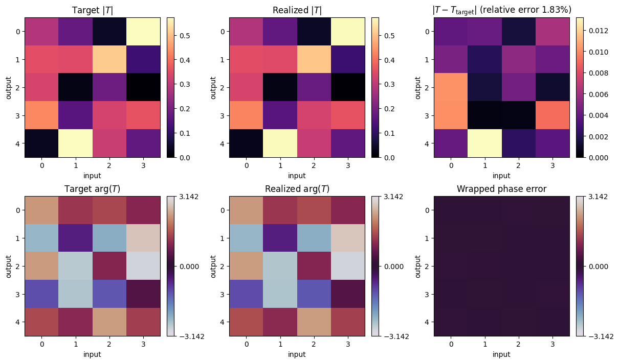
We first compare the target and realized transmission matrices in amplitude and phase. The optimization history then shows how the transmission error, reflection, fabrication penalty, and classifier accuracy change over the 50 updates.
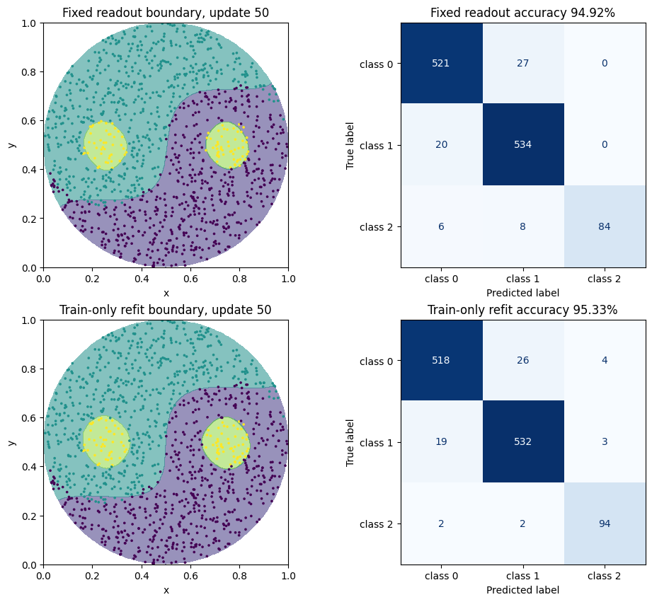
For the main evaluation, we keep the electronic readout learned with the target matrix fixed. Its held-out accuracy therefore measures how well the inverse-designed silicon device reproduces the intended optical transformation. We also report a readout refitted using only the realized training-set powers. This second result shows how much accuracy can be recovered electronically without changing the optical device; the held-out set remains reserved for final evaluation.
cache_available = PROGRESS_PATH.exists()
if cache_available:
    with np.load(PROGRESS_PATH, allow_pickle=False) as saved:
        updates_completed = int(saved["update"])
        rows = [
            {
                "loss": -float(saved["score_history"][index]),
                "T": float(saved["transmission_loss_history"][index]),
                "R": float(saved["reflection_loss_history"][index]),
                "fab": float(saved["fabrication_penalty_history"][index]),
                "weight": float(saved["fabrication_weight_history"][index]),
                "beta": float(saved["projection_beta_history"][index]),
                "gray_01_99": float(saved["gray_fraction_01_99_history"][index]),
                "gray_10_90": float(saved["gray_fraction_10_90_history"][index]),
                "accuracy": float(saved["realized_accuracy_history"][index]),
                "CE": float(saved["realized_ce_loss_history"][index]),
                "minimum_insertion_loss_db": float(
                    saved["minimum_insertion_loss_db_history"][index]
                ),
                "minimum_output_row_power": float(
                    saved["minimum_output_row_power_history"][index]
                ),
            }
            for index in range(updates_completed)
        ]
        final_parameters = np.asarray(saved["parameters_before"])[..., 0]
        final_transmission = np.asarray(saved["transmission"])
    transmission_residual = final_transmission - target_matrix
    relative_transmission_error = np.linalg.norm(
        transmission_residual
    ) / np.linalg.norm(target_matrix)
    wrapped_phase_error = np.angle(final_transmission * np.conj(target_matrix))
    magnitude_limit = max(
        np.max(np.abs(target_matrix)),
        np.max(np.abs(final_transmission)),
    )

    fig, axes = plt.subplots(2, 3, figsize=(12, 7), constrained_layout=True)
    for axis, matrix, title in (
        (axes[0, 0], np.abs(target_matrix), r"Target $|T|$"),
        (axes[0, 1], np.abs(final_transmission), r"Realized $|T|$"),
    ):
        image = axis.imshow(
            matrix,
            cmap="magma",
            aspect="auto",
            vmin=0,
            vmax=magnitude_limit,
        )
        fig.colorbar(image, ax=axis)
        axis.set_title(title)
    residual_image = axes[0, 2].imshow(
        np.abs(transmission_residual),
        cmap="magma",
        aspect="auto",
        vmin=0,
    )
    fig.colorbar(residual_image, ax=axes[0, 2])
    axes[0, 2].set_title(
        r"$|T-T_{\mathrm{target}}|$"
        f" (relative error {relative_transmission_error:.2%})"
    )
    for axis, matrix, title in (
        (axes[1, 0], np.angle(target_matrix), r"Target $\arg(T)$"),
        (
            axes[1, 1],
            np.angle(final_transmission),
            r"Realized $\arg(T)$",
        ),
        (
            axes[1, 2],
            wrapped_phase_error,
            "Wrapped phase error",
        ),
    ):
        image = axis.imshow(
            matrix,
            cmap="twilight",
            aspect="auto",
            vmin=-np.pi,
            vmax=np.pi,
        )
        fig.colorbar(image, ax=axis, ticks=(-np.pi, 0, np.pi))
        axis.set_title(title)
    for axis in axes.flat:
        axis.set(xlabel="input", ylabel="output")
else:
    print(
        "No realization cache is present. "
        "The trained target and validated inverse-design model are ready."
    )
if cache_available:
    updates = np.arange(1, len(rows) + 1)
    fig, axes = plt.subplots(2, 4, figsize=(16, 7), constrained_layout=True)
    axes[0, 0].plot(
        updates,
        [row["loss"] for row in rows],
        marker="o",
        label="total physical loss",
    )
    axes[0, 0].plot(
        updates,
        [row["T"] for row in rows],
        marker="o",
        label=r"$\|T-T_{target}\|_F$",
    )
    axes[0, 0].set(title="Loss and target error", ylabel="value")
    axes[0, 0].legend(frameon=False)
    axes[0, 1].plot(updates, [row["R"] for row in rows], marker="o")
    axes[0, 1].set(title="Reflection", ylabel=r"$\|R\|_F$")
    axes[0, 2].plot(
        updates,
        [row["weight"] * row["fab"] for row in rows],
        marker="o",
    )
    axes[0, 2].set(title="Weighted fabrication penalty")
    axes[0, 3].plot(
        updates,
        [row["accuracy"] for row in rows],
        marker="o",
    )
    axes[0, 3].set(title="Realized accuracy", ylabel="accuracy")
    axes[0, 3].set_ylim(0, 1)
    axes[1, 0].plot(
        updates,
        [row["CE"] for row in rows],
        marker="o",
    )
    axes[1, 0].set(title="Realized cross-entropy", ylabel="CE loss")
    axes[1, 1].imshow(final_parameters, origin="lower", cmap="gray")
    axes[1, 1].set(title=f"Cached design after {updates_completed} updates")
    axes[1, 2].imshow(np.abs(final_transmission), cmap="magma", aspect="auto")
    axes[1, 2].set(
        title=(
            r"Realized $|T|$"
            f" (min row power {rows[-1]['minimum_output_row_power']:.3f})"
        )
    )
    axes[1, 3].plot(
        updates,
        [row["minimum_insertion_loss_db"] for row in rows],
        marker="o",
        label="minimum over inputs",
    )
    axes[1, 3].axhline(
        MINIMUM_INSERTION_LOSS_DB,
        color="black",
        linestyle="--",
        label="3 dB requirement",
    )
    axes[1, 3].set(title="Realized insertion loss", ylabel="insertion loss (dB)")
    axes[1, 3].legend(frameon=False)
    for axis in axes.flat:
        axis.set_xlabel("update")
        axis.grid(alpha=0.2)
if cache_available:
    realized_train_powers = np.abs(train_x @ final_transmission.T) ** 2
    realized_test_powers = np.abs(test_x @ final_transmission.T) ** 2
    realized_logits = realized_test_powers @ readout_w + readout_b
    realized_prediction = np.argmax(realized_logits, axis=1)
    fixed_accuracy = np.mean(realized_prediction == test_y)

    refit_readout = LogisticRegression(
        C=np.inf,
        solver="lbfgs",
        max_iter=5000,
        random_state=DATA_SEED,
    )
    refit_readout.fit(realized_train_powers, train_y)
    refit_prediction = refit_readout.predict(realized_test_powers)
    refit_probability = refit_readout.predict_proba(realized_test_powers)
    refit_accuracy = np.mean(refit_prediction == test_y)
    refit_ce = log_loss(
        test_y,
        refit_probability,
        labels=np.arange(N_CLASSES),
    )
    print(
        f"update {len(rows)} fixed readout: "
        f"accuracy={fixed_accuracy:.2%}, CE={rows[-1]['CE']:.6f}"
    )
    print(
        f"update {len(rows)} train-only refit: "
        f"accuracy={refit_accuracy:.2%}, CE={refit_ce:.6f}"
    )
update 50 fixed readout: accuracy=94.92%, CE=0.175041
update 50 train-only refit: accuracy=95.33%, CE=0.108883
/Users/jungmin/miniconda3/envs/test/lib/python3.13/site-packages/sklearn/linear_model/_logistic.py:1170: UserWarning: Setting penalty=None will ignore the C and l1_ratio parameters
  warnings.warn(
if cache_available:
    grid_axis = np.linspace(0.0, 1.0, 401)
    grid_x, grid_y = np.meshgrid(grid_axis, grid_axis)
    grid_raw = np.column_stack(
        (
            grid_x.ravel(),
            grid_y.ravel(),
            1.0 - grid_x.ravel(),
            1.0 - grid_y.ravel(),
        )
    )
    grid_fields = encode(grid_raw)
    grid_powers = np.abs(grid_fields @ final_transmission.T) ** 2
    fixed_grid_logits = grid_powers @ readout_w + readout_b
    fixed_grid_prediction = np.argmax(fixed_grid_logits, axis=1).reshape(grid_x.shape)
    refit_grid_prediction = refit_readout.predict(grid_powers).reshape(grid_x.shape)
    disk = (grid_x - 0.5) ** 2 + (grid_y - 0.5) ** 2 <= 0.25
    fixed_grid_prediction = np.ma.masked_where(~disk, fixed_grid_prediction)
    refit_grid_prediction = np.ma.masked_where(~disk, refit_grid_prediction)

    fig, axes = plt.subplots(2, 2, figsize=(10, 8.4), constrained_layout=True)
    for axis, prediction, title in (
        (
            axes[0, 0],
            fixed_grid_prediction,
            f"Fixed readout boundary, update {len(rows)}",
        ),
        (
            axes[1, 0],
            refit_grid_prediction,
            f"Train-only refit boundary, update {len(rows)}",
        ),
    ):
        axis.contourf(
            grid_x,
            grid_y,
            prediction,
            levels=(-0.5, 0.5, 1.5, 2.5),
            cmap="viridis",
            alpha=0.55,
        )
        axis.scatter(
            raw_features[test_indices, 0],
            raw_features[test_indices, 1],
            c=test_y,
            cmap="viridis",
            vmin=0,
            vmax=N_CLASSES - 1,
            s=7,
            linewidths=0,
        )
        axis.set(
            title=title,
            xlabel="x",
            ylabel="y",
            aspect="equal",
            xlim=(0, 1),
            ylim=(0, 1),
        )
    for axis, prediction, title in (
        (
            axes[0, 1],
            realized_prediction,
            f"Fixed readout accuracy {fixed_accuracy:.2%}",
        ),
        (
            axes[1, 1],
            refit_prediction,
            f"Train-only refit accuracy {refit_accuracy:.2%}",
        ),
    ):
        ConfusionMatrixDisplay(
            confusion_matrix(test_y, prediction),
            display_labels=("class 0", "class 1", "class 2"),
        ).plot(ax=axis, colorbar=False, cmap="Blues")
        axis.set_title(title)
Visualize the Realized Device
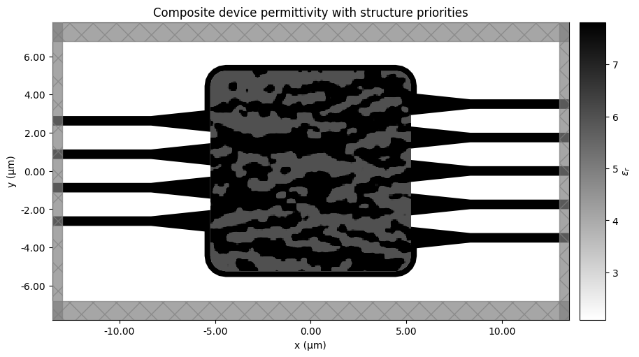
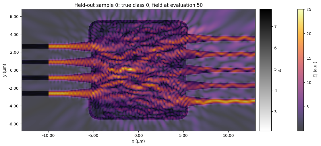
We first plot the final permittivity distribution, including the optimized region and fixed input and output structures. We can then optionally excite the device with one held-out sample and visualize the combined electric-field magnitude.
The field calculation requires a new cloud simulation, fresh cost estimate, and explicit approval through COST_APPROVED=True.
if cache_available:
    with np.load(PROGRESS_PATH, allow_pickle=False) as saved:
        display_parameters = np.asarray(saved["parameters_before"])
        display_beta = float(saved["projection_beta_history"][-1])
    display_factory = build_modal_factory(calibration, projection_beta=display_beta)
    display_modeler = display_factory.modeler(display_parameters)
    display_simulation = next(iter(display_modeler.sim_dict.values()))
    fig, ax = plt.subplots(figsize=(11, 5), constrained_layout=True)
    display_simulation.plot_eps(
        z=0,
        ax=ax,
        source_alpha=0,
        monitor_alpha=0,
    )
    ax.set(
        title="Composite device permittivity with structure priorities",
        xlabel="x (µm)",
        ylabel="y (µm)",
    )
else:
    print("No realization cache is available for a permittivity plot.")
sample_data = None
sample_index = int(SINGLE_SAMPLE_INDEX)
sample_field_evaluation = updates_completed if cache_available else 0
field_path = OUTPUT_DIR / (
    f"single_sample_field_update_{sample_field_evaluation:03d}.hdf5"
)
coordinates = device_coordinates()
x0, x1 = coordinates["domain_x"]
y0, y1 = coordinates["domain_y"]

if RUN_SINGLE_SAMPLE_FIELD:
    if not cache_available:
        raise ValueError("A realization checkpoint is required.")
    sample_field_evaluation = updates_completed if cache_available else 0
    if fresh_forward_cost is None or not COST_APPROVED:
        raise ValueError("Run a fresh estimate and set COST_APPROVED=True first.")
    if not 0 <= sample_index < len(test_x):
        raise IndexError("SINGLE_SAMPLE_INDEX is outside the test set.")

    sample_modeler = display_factory.modeler(display_parameters)
    source_simulations = list(sample_modeler.sim_dict.values())
    base_simulation = source_simulations[0]
    sample_sources = []
    for input_index, coefficient in enumerate(test_x[sample_index]):
        source = source_simulations[input_index].sources[0]
        pulse = source.source_time.updated_copy(
            amplitude=float(np.abs(coefficient)),
            phase=float(np.angle(coefficient)),
        )
        sample_sources.append(
            source.updated_copy(
                source_time=pulse,
                name=f"sample_input_{input_index:02d}",
            )
        )

    field_monitor = td.FieldMonitor(
        center=((x0 + x1) / 2, (y0 + y1) / 2, 0),
        size=(x1 - x0, y1 - y0, 0),
        freqs=[FREQUENCY_HZ],
        fields=("Ex", "Ey", "Ez"),
        name="sample_field",
        colocate=True,
    )
    sample_simulation = base_simulation.updated_copy(
        sources=tuple(sample_sources),
        monitors=base_simulation.monitors + (field_monitor,),
    )
    sample_simulation.validate_pre_upload()
    sample_data = web.run(
        sample_simulation,
        task_name="classifier_single_sample_field",
        folder_name="classifier_field",
        path=field_path,
        verbose=False,
    )
elif field_path.exists():
    sample_data = td.SimulationData.from_file(field_path)

if sample_data is not None:
    field = sample_data["sample_field"]
    ex = np.asarray(field.Ex.sel(f=FREQUENCY_HZ, method="nearest").squeeze())
    ey = np.asarray(field.Ey.sel(f=FREQUENCY_HZ, method="nearest").squeeze())
    ez = np.asarray(field.Ez.sel(f=FREQUENCY_HZ, method="nearest").squeeze())
    magnitude = np.sqrt(np.abs(ex) ** 2 + np.abs(ey) ** 2 + np.abs(ez) ** 2)
    field_x = np.asarray(field.Ex.coords["x"])
    field_y = np.asarray(field.Ex.coords["y"])

    fig, ax = plt.subplots(figsize=(11, 5), constrained_layout=True)
    sample_data.simulation.plot_eps(
        z=0,
        ax=ax,
        alpha=0.82,
        source_alpha=0,
        monitor_alpha=0,
    )
    overlay = ax.pcolormesh(
        field_x,
        field_y,
        magnitude.T,
        shading="auto",
        cmap="inferno",
        alpha=0.72,
    )
    fig.colorbar(overlay, ax=ax, label=r"$|E|$ (a.u.)")
    ax.set(
        title=(
            f"Held-out sample {sample_index}: "
            f"true class {test_y[sample_index]}, "
            f"field at evaluation {sample_field_evaluation}"
        ),
        xlabel="x (µm)",
        ylabel="y (µm)",
        xlim=(x0, x1),
        ylim=(y0, y1),
    )
else:
    print(
        "Single-sample field simulation is disabled and no cached field "
        "data is present."
    )
Summary
We trained a passive 5 × 4 optical transformation together with a 5 × 3 electronic readout, then fixed the optical target and transferred it to a four-input, five-output inverse-designed silicon device. The realization objective matches the complete complex transmission matrix while suppressing reflection and penalizing sub-200 nm features.
The final plots compare the target and realized responses, track the optimization history, and evaluate the classifier with both the original and refitted electronic readouts.
This notebook uses a two-dimensional effective-index model, which does not capture out-of-plane scattering. For a fabrication-level device, three-dimensional optimization is strongly recommended, either from scratch or by fine-tuning this design.
References
-
A. M. I. Muda and U. Teğin, “Scalable photonic neural networks via surrogate scattering-matrix inverse design,” arXiv:2604.21301 [physics.optics] (2026). arXiv:2604.21301
-
Flexcompute, Inverse design overview.
-
Flexcompute, Effective index approximation in Tidy3D.
-
V. Nikkhah et al., “Inverse-designed low-index-contrast structures on a silicon photonics platform for vector–matrix multiplication,” Nature Photonics 18, 501–508 (2024). doi:10.1038/s41566-024-01394-2


 TERMS & CONDITIONS


 How the process works:
 Try this real URL to see an example: