





Author: Marcus Ossiander, Graz University of Technology
This example uses a custom source in Tidy3D FDTD to compare sum frequency generation in lithium niobate and a novel multi-quantum-well material.
See our paper preprint at https://arxiv.org/abs/2604.15476
Quantum-Well-Metasurface to Maximize Nonlinear Polarization
P. Fathi, I. Occhiodori, P. Devaney, A. Ricks, R. Ramesh, Y. Ju, M. Waqar, T. Letsou, C. Spägele, H. Jung, I. Brener, X. Pan, M. Ossiander, S. Bank, F. Capasso*
See https://github.com/marcus-o/linbo_mqw_comparison for the data files.
import tidy3d as td
import numpy as np
import tidy3d.web as web
import matplotlib.pyplot as plt
from tqdm import tqdm

c = 3e8  # (m/sec)
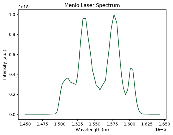
Load the input laser spectrum (no spectral phase included). This data has reduced resolution for brevity.
wls_menlo = np.array(
      [1.45000000e-06, 1.45406056e-06, 1.45718823e-06, 1.45917310e-06,
       1.46115797e-06, 1.46314284e-06, 1.46512771e-06, 1.46684192e-06,
       1.46936811e-06, 1.47338561e-06, 1.47726658e-06, 1.48226976e-06,
       1.48274342e-06, 1.48384067e-06, 1.48479596e-06, 1.48577550e-06,
       1.48714171e-06, 1.48986840e-06, 1.49312913e-06, 1.49376396e-06,
       1.49426920e-06, 1.49463008e-06, 1.49499097e-06, 1.49562252e-06,
       1.49624404e-06, 1.49702596e-06, 1.49751716e-06, 1.49850960e-06,
       1.49959225e-06, 1.50116210e-06, 1.50356199e-06, 1.50753173e-06,
       1.51150147e-06, 1.51518250e-06, 1.51908006e-06, 1.52304980e-06,
       1.52539555e-06, 1.52756086e-06, 1.52959986e-06, 1.53315458e-06,
       1.53712432e-06, 1.54038617e-06, 1.54416159e-06, 1.54668778e-06,
       1.54939442e-06, 1.55203662e-06, 1.55488289e-06, 1.55754441e-06,
       1.56151791e-06, 1.56553115e-06, 1.56763918e-06, 1.57068665e-06,
       1.57375418e-06, 1.57772392e-06, 1.58169365e-06, 1.58470103e-06,
       1.58697160e-06, 1.58891136e-06, 1.59107667e-06, 1.59414420e-06,
       1.59730194e-06, 1.59896201e-06, 1.60118146e-06, 1.60470009e-06,
       1.60685538e-06, 1.60821872e-06, 1.60939160e-06, 1.61036148e-06,
       1.61146669e-06, 1.61250925e-06, 1.61327112e-06, 1.61408311e-06,
       1.61480488e-06, 1.61539132e-06, 1.61611309e-06, 1.61678975e-06,
       1.61751152e-06, 1.61830346e-06, 1.61895506e-06, 1.61970690e-06,
       1.62164881e-06, 1.62479940e-06, 1.62656372e-06, 1.62738574e-06,
       1.62876913e-06, 1.62924029e-06, 1.62987184e-06, 1.63051341e-06,
       1.63127671e-06, 1.63361602e-06, 1.63483401e-06, 1.64107733e-06,
       1.64300000e-06])
intensity_menlo = np.array(
      [0.00000000e+00, 1.07397406e+14, 1.73730016e+14, 1.73836425e+14,
       1.73836425e+14, 1.73836425e+14, 1.73836425e+14, 1.73836425e+14,
       1.09221120e+14, 1.08487947e+14, 1.08820595e+14, 2.56728134e+14,
       3.96706703e+14, 5.63869590e+14, 8.44209129e+14, 1.16040697e+15,
       1.62905171e+15, 2.26857894e+15, 2.94958017e+15, 4.54325989e+15,
       7.12629752e+15, 1.06392091e+16, 1.53233611e+16, 2.22893694e+16,
       3.35714027e+16, 5.42380341e+16, 7.74191594e+16, 1.10507808e+17,
       1.59698272e+17, 2.32396782e+17, 3.04868784e+17, 3.46489820e+17,
       3.63217202e+17, 3.21530005e+17, 3.09192638e+17, 2.98039534e+17,
       3.85266564e+17, 5.34518398e+17, 7.21501822e+17, 9.56871626e+17,
       9.59805607e+17, 7.75499200e+17, 6.01037172e+17, 4.44549770e+17,
       3.70404186e+17, 2.94206012e+17, 2.74030155e+17, 2.43835007e+17,
       2.95021004e+17, 3.39558872e+17, 4.82333023e+17, 6.53408526e+17,
       8.61749736e+17, 9.98164768e+17, 9.16164110e+17, 6.73447235e+17,
       4.98899752e+17, 3.69799877e+17, 2.66446674e+17, 1.97020390e+17,
       2.40680442e+17, 3.30087839e+17, 4.60809154e+17, 4.49442079e+17,
       3.15074755e+17, 2.29557636e+17, 1.66657959e+17, 1.18439742e+17,
       8.29062556e+16, 5.81039017e+16, 4.15215613e+16, 3.02207276e+16,
       2.20946052e+16, 1.60631222e+16, 1.14413271e+16, 8.19751715e+15,
       5.59346665e+15, 3.77508236e+15, 2.59328520e+15, 1.76618611e+15,
       1.41615465e+15, 1.49136220e+15, 1.07660717e+15, 7.43009562e+14,
       4.78862411e+14, 3.36899408e+14, 2.27148743e+14, 1.60219058e+14,
       1.14383841e+14, 1.26239998e+14, 1.34581616e+14, 1.02727783e+14,
       0.00000000e+00])

# plot the spectrum
plt.plot(wls_menlo, intensity_menlo)
plt.xlabel('Wavelength (m)')
plt.ylabel('Intensity (a.u.)')
plt.title('Menlo Laser Spectrum')
plt.show()
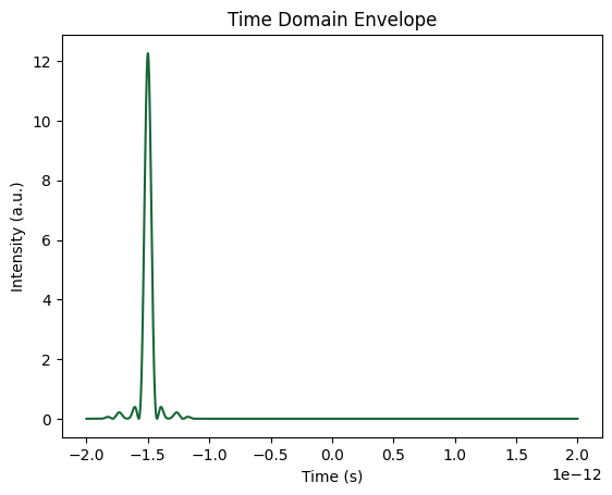
Convert the spectrum to the frequency and then the time domain, then split it into center frequency and envelope to use in Tidy3D:
wls_fund = wls_menlo
intensity_wls = intensity_menlo
freqs_fund = c / wls_fund
intensity_f_fund = intensity_wls*(c/freqs_fund**2)

# create time domain pulse via fft to use in a tidy3d source
dt = 0.2e-15  # time step in seconds
time = np.arange(-2000e-15, 2000e-15, dt)
time = time - time[time.size//2]  # ensure there is a proper 0 time point

freqs = np.fft.fftfreq(len(time), time[1]-time[0])
e_fd = np.zeros_like(freqs)
e_fd[freqs > 0] = np.interp(
    freqs[freqs > 0],
    freqs_fund[::-1],
    np.sqrt(intensity_f_fund[::-1]))

# tidy3d needs the envelope and the center frequency
center_freq = np.sum(freqs*np.abs(e_fd)**2) / np.sum(np.abs(e_fd)**2)
center_freq_idx = np.argmin(np.abs(freqs - center_freq))
center_freq = freqs[center_freq_idx]

# this allows one to add gdd (chirp) but our output shg spectrum
# matches well, so no significant chirping of the pulse is expected
# furthermore, the measurement was done with minimal dispersion
# in the path after the compression unit
gd = - 1500e-15
gdd = 0.e-30
tod = 0.e-45
fod = 0.e-60
e_fd = e_fd * np.exp(
    1j*gd*2*np.pi*(freqs-center_freq)
    + 1j*gdd*2*np.pi*(freqs-center_freq)**2
    + 1j*tod*2*np.pi*(freqs-center_freq)**3
    + 1j*fod*2*np.pi*(freqs-center_freq)**4)

# shift to center frequency at zero index
e_fd = np.roll(e_fd, -center_freq_idx)
e_td = np.fft.fftshift(np.fft.fft(e_fd))

# plot time domain pulse
plt.plot(time, np.real(e_td)**2)
plt.xlabel('Time (s)')
plt.ylabel('Intensity (a.u.)')
plt.title('Time Domain Envelope')
plt.show()
Create a tidy3d simulation for a thin nonlinear layer bonded using glue to a substrate (the layer is linear in the simulation):
def get_fields_tidy(
        ref,
        aoi_deg,
        layer_thickness_um, epoxy_thickness_um, substrate_thickness_um,
        layer_index, epoxy_index, substrate_index):

    # materials (narrowband is fine as our relative bandwidth is small)
    vacuum_material = td.Medium(name='Vacuum')
    layer_material = td.Medium(
        name='layer', permittivity=layer_index**2)
    epoxy_material = td.Medium(
        name='epoxy', permittivity=epoxy_index**2)
    substrate_material = td.Medium(
        name='substrate', permittivity=substrate_index**2)

    # total simulation size
    tx = 1  # um
    tz = 2 + substrate_thickness_um + epoxy_thickness_um + layer_thickness_um + 2  # um

    # source with the custom spectrum
    source = td.PlaneWave(
        name='planewave_0',
        center=[0, 0, -substrate_thickness_um-1],
        size=[10, 10, 0],
        source_time=td.CustomSourceTime.from_values(
            center_freq, np.std(np.abs(e_fd)), values=e_td, dt=dt),
        direction='+',
        angle_theta=aoi_deg/180*np.pi)

    # structures: substrate, epoxy, nonlinear layer
    substrate = td.Structure(
        geometry=td.Box(
            center=[0, 0, -substrate_thickness_um/2],
            size=[4, 4, substrate_thickness_um]),
        name='substrate',
        medium=substrate_material)

    epoxy = td.Structure(
        geometry=td.Box(
            center=[0, 0, epoxy_thickness_um/2],
            size=[10, 10, epoxy_thickness_um]),
        name='epoxy',
        medium=epoxy_material)

    layer = td.Structure(
        geometry=td.Box(
            center=[0, 0, epoxy_thickness_um+layer_thickness_um/2],
            size=[10, 10, layer_thickness_um]),
        name='layer',
        medium=layer_material)

    # record the fields in the nonlinear layer
    fieldtimemonitor_layer = td.FieldTimeMonitor(
        name='fieldtimemonitor_layer',
        center=[0, 0, epoxy_thickness_um+layer_thickness_um/2],
        size=[0, 0, 0],
        interval=2)

    # allow running with or without the structures for reference
    if not ref:
        structures = [substrate, epoxy, layer]
    else:
        structures = []

    # boundaries:
    # x: Bloch from source as there can be an incidence angle
    # y: periodic
    # z: PML
    bloch_boundary_x = td.Boundary.bloch_from_source(
        source=source, domain_size=tx, axis=0)
    periodic_boundary_y = td.Boundary(
            plus=td.Periodic(), minus=td.Periodic())
    pml_boundary_z = td.Boundary(
        plus=td.PML(parameters=td.PMLParams(
            kappa_min=1, kappa_max=3, alpha_order=1, alpha_max=0)),
        minus=td.PML(parameters=td.PMLParams(
            kappa_min=1, kappa_max=3, alpha_order=1, alpha_max=0)
            ), )

    # create and run simulation
    sim = td.Simulation(
        center=[0, 0, layer_thickness_um+epoxy_thickness_um+2-tz/2],
        size=[tx, 0, tz],
        boundary_spec=td.BoundarySpec(
            x=bloch_boundary_x, y=periodic_boundary_y, z=pml_boundary_z),
        grid_spec=td.GridSpec(wavelength=1.550),
        run_time=6e-12,
        medium=vacuum_material,
        sources=[source],
        monitors=[fieldtimemonitor_layer],
        structures=structures,
        shutoff=0)
    data = web.run(sim, task_name='mqw_sim', path='./ln_comp/data/prop_inside.hdf5')
    return data
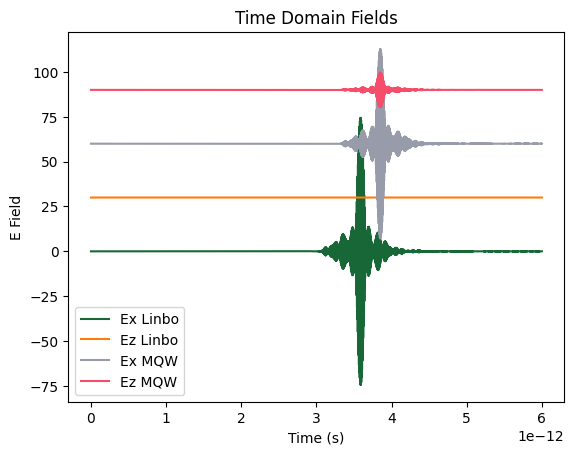
Get the time domain fields in the center of a thin film of lithium niobate and a thin film of a multi-quantum-well material:
# %%
# Lithium niobate bonded to alumina (sapphire) substrate, without epoxy resin
ref = False
aoi_deg = 0
layer_thickness_um = 0.6
epoxy_thickness_um = 0.1
substrate_thickness_um = 500
# there is no epoxy in the linbo sample, so the epoxy layer is given
# the sapphire index and becomes optically part of the substrate
epoxy_index = 1.76  # sapphire refractive index
layer_index = 2.1373  # linbo
substrate_index = 1.76  # sapphire

# run the linbo simulation
data_linbo = get_fields_tidy(
    ref,
    aoi_deg, layer_thickness_um, epoxy_thickness_um, substrate_thickness_um,
    layer_index, epoxy_index, substrate_index)

# A nonlinear MQW bonded to alumina with epoxy resin
ref = False
aoi_deg = 45
layer_thickness_um = 0.595
epoxy_thickness_um = 0.5
substrate_thickness_um = 500
layer_index = 3.175474  # mqw index
epoxy_index = 1.56  # epoxy resin
substrate_index = 1.76  # sapphire

# run the mqw simulation
data_mqw = get_fields_tidy(
    ref,
    aoi_deg, layer_thickness_um, epoxy_thickness_um, substrate_thickness_um,
    layer_index, epoxy_index, substrate_index)

# %% extract the time domain field along different directions in the center of the nonlinear layers
t_linbo = np.real(np.array(
    data_linbo.monitor_data['fieldtimemonitor_layer'].Ex.t))
etx_linbo = np.real(
    data_linbo.monitor_data['fieldtimemonitor_layer'].Ex[0, 0, 0, :])
etz_linbo = np.real(
    data_linbo.monitor_data['fieldtimemonitor_layer'].Ez[0, 0, 0, :])

t_mqw = np.real(np.array(
    data_mqw.monitor_data['fieldtimemonitor_layer'].Ex.t))
etx_mqw = np.real(
    data_mqw.monitor_data['fieldtimemonitor_layer'].Ex[0, 0, 0, :])
etz_mqw = np.real(
    data_mqw.monitor_data['fieldtimemonitor_layer'].Ez[0, 0, 0, :])

# %% plot fields
plt.plot(t_linbo, 0+etx_linbo)
plt.plot(t_linbo, 30+etz_linbo)
plt.plot(t_mqw, 60+etx_mqw)
plt.plot(t_mqw, 90+etz_mqw)
plt.xlabel('Time (s)')
plt.ylabel('E Field')
plt.title('Time Domain Fields')
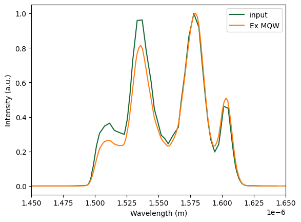
plt.legend(['Ex Linbo', 'Ez Linbo', 'Ex MQW', 'Ez MQW'])
plt.show()

# %% plot spectra to see if there are strong interference effects
freqs_td = np.fft.fftfreq(t_mqw.size, t_mqw[1] - t_mqw[0])
e_f_td = np.fft.ifft(etx_mqw)
plt.plot(wls_menlo, intensity_menlo/np.max(intensity_menlo))
plt.plot(c/(freqs_td+1), np.abs(e_f_td)**2/np.max(np.abs(e_f_td)**2))
plt.xlim(1450e-9, 1650e-9)
plt.xlabel('Wavelength (m)')
plt.ylabel('Intensity (a.u.)')
plt.legend(['input', 'Ex MQW'])
plt.show()
09:42:30 EDT WARNING: 'normalize_index' 0 is a source with 'CustomSourceTime'
             time dependence. Normalizing frequency-domain monitors by this
             source is only meaningful if field decay occurs.
09:42:31 EDT Created task 'mqw_sim' with resource_id
             'fdve-90cd3305-62ce-4eb2-8a8b-f9826a9b3614' and task_type 'FDTD'.
             View task using web UI at
             'https://tidy3d.simulation.cloud/workbench?taskId=fdve-90cd3305-62c
             e-4eb2-8a8b-f9826a9b3614'.
Task folder: 'default'.
Output()
09:42:33 EDT Estimated FlexCredit cost: 0.025. Minimum cost depends on task
             execution details. Use 'web.real_cost(task_id)' to get the billed
             FlexCredit cost after a simulation run.
09:42:34 EDT status = queued
             To cancel the simulation, use 'web.abort(task_id)' or
             'web.delete(task_id)' or abort/delete the task in the web UI.
             Terminating the Python script will not stop the job running on the
             cloud.
Output()
09:42:41 EDT status = preprocess
09:42:46 EDT starting up solver
running solver
Output()
09:42:50 EDT status = postprocess
Output()
09:42:53 EDT status = success
09:42:55 EDT View simulation result at
             'https://tidy3d.simulation.cloud/workbench?taskId=fdve-90cd3305-62c
             e-4eb2-8a8b-f9826a9b3614'.
Output()
09:42:57 EDT Loading simulation from ln_comp/data/prop_inside.hdf5
             WARNING: 'normalize_index' 0 is a source with 'CustomSourceTime'
             time dependence. Normalizing frequency-domain monitors by this
             source is only meaningful if field decay occurs.
             WARNING: Warning messages were found in the solver log. For more
             information, check 'SimulationData.log' or use
             'web.download_log(task_id)'.
             WARNING: 'normalize_index' 0 is a source with 'CustomSourceTime'
             time dependence. Normalizing frequency-domain monitors by this
             source is only meaningful if field decay occurs.
             Created task 'mqw_sim' with resource_id
             'fdve-aee8eba2-bf96-4ecb-811d-d010cbfbc9d3' and task_type 'FDTD'.
             View task using web UI at
             'https://tidy3d.simulation.cloud/workbench?taskId=fdve-aee8eba2-bf9
             6-4ecb-811d-d010cbfbc9d3'.
Task folder: 'default'.
Output()
09:42:59 EDT Estimated FlexCredit cost: 0.025. Minimum cost depends on task
             execution details. Use 'web.real_cost(task_id)' to get the billed
             FlexCredit cost after a simulation run.
09:43:00 EDT status = queued
             To cancel the simulation, use 'web.abort(task_id)' or
             'web.delete(task_id)' or abort/delete the task in the web UI.
             Terminating the Python script will not stop the job running on the
             cloud.
Output()
09:43:10 EDT starting up solver
running solver
Output()
09:43:17 EDT status = postprocess
Output()
09:43:20 EDT status = success
09:43:22 EDT View simulation result at
             'https://tidy3d.simulation.cloud/workbench?taskId=fdve-aee8eba2-bf9
             6-4ecb-811d-d010cbfbc9d3'.
Output()
09:43:23 EDT Loading simulation from ln_comp/data/prop_inside.hdf5
             WARNING: 'normalize_index' 0 is a source with 'CustomSourceTime'
             time dependence. Normalizing frequency-domain monitors by this
             source is only meaningful if field decay occurs.
             WARNING: Warning messages were found in the solver log. For more
             information, check 'SimulationData.log' or use
             'web.download_log(task_id)'.
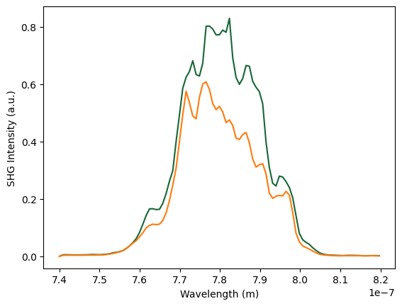
Load the measured SFG data for linbo at 0 deg and mqw at 45 deg angles of incidence; otherwise, the data are comparable (same experimental conditions). This data has reduced resolution for brevity.
wls_shg = np.array(
      [7.40007957e-07, 7.40839072e-07, 7.41670310e-07, 7.42501304e-07,
       7.43332419e-07, 7.44163413e-07, 7.44994407e-07, 7.45825400e-07,
       7.46656333e-07, 7.47487266e-07, 7.48318198e-07, 7.49149009e-07,
       7.49979880e-07, 7.50810630e-07, 7.51641440e-07, 7.52472190e-07,
       7.53302878e-07, 7.54133567e-07, 7.54964194e-07, 7.55794822e-07,
       7.56625449e-07, 7.57456016e-07, 7.58286521e-07, 7.59117026e-07,
       7.59947593e-07, 7.60777976e-07, 7.61608298e-07, 7.62438743e-07,
       7.63269126e-07, 7.64099387e-07, 7.64929709e-07, 7.65759971e-07,
       7.66590232e-07, 7.67420371e-07, 7.68250571e-07, 7.69080710e-07,
       7.69910850e-07, 7.70740928e-07, 7.71570945e-07, 7.72400901e-07,
       7.73230918e-07, 7.74060874e-07, 7.74890830e-07, 7.75720725e-07,
       7.76550620e-07, 7.77380393e-07, 7.78210227e-07, 7.79040000e-07,
       7.79869712e-07, 7.80699363e-07, 7.81529075e-07, 7.82358787e-07,
       7.83188438e-07, 7.84017966e-07, 7.84847556e-07, 7.85677024e-07,
       7.86506492e-07, 7.87336021e-07, 7.88165427e-07, 7.88994712e-07,
       7.89824180e-07, 7.90653525e-07, 7.91482810e-07, 7.92312034e-07,
       7.93141318e-07, 7.93970542e-07, 7.94799644e-07, 7.95628806e-07,
       7.96457908e-07, 7.97287009e-07, 7.98116050e-07, 7.98945090e-07,
       7.99774070e-07, 8.00602988e-07, 8.01431968e-07, 8.02260764e-07,
       8.03089622e-07, 8.03918540e-07, 8.04747214e-07, 8.05575950e-07,
       8.06404746e-07, 8.07233420e-07, 8.08062095e-07, 8.08890708e-07,
       8.09719321e-07, 8.10547874e-07, 8.11376426e-07, 8.12204917e-07,
       8.13033286e-07, 8.13861777e-07, 8.14690208e-07, 8.15518577e-07,
       8.16346885e-07, 8.17175132e-07, 8.18003501e-07, 8.18831687e-07,
       8.19659873e-07])

intensity_mqw_meas = np.array(
      [0.        , 0.00523578, 0.00560511, 0.00532924, 0.00516043,
       0.0048538 , 0.00488337, 0.00528942, 0.00535738, 0.00597015,
       0.00641102, 0.00596538, 0.00575818, 0.00634449, 0.00745703,
       0.00894295, 0.01203258, 0.01415894, 0.01590141, 0.0198475 ,
       0.02707253, 0.03629635, 0.04754925, 0.06137581, 0.08288472,
       0.11160864, 0.14203952, 0.16557082, 0.16617025, 0.1632654 ,
       0.16403388, 0.18483773, 0.2190888 , 0.26219245, 0.29898499,
       0.40099785, 0.49324993, 0.5865733 , 0.62496787, 0.64482991,
       0.68218658, 0.63439603, 0.62887652, 0.67390171, 0.80245468,
       0.80302907, 0.7926517 , 0.77241674, 0.772999  , 0.7891274 ,
       0.78151635, 0.82999764, 0.69241303, 0.62377022, 0.60005055,
       0.62037634, 0.66566047, 0.66293422, 0.6101542 , 0.58990255,
       0.57422837, 0.53201551, 0.39852695, 0.30956216, 0.25512455,
       0.24525909, 0.27989213, 0.27672859, 0.26080452, 0.24051044,
       0.20521002, 0.14276436, 0.08060076, 0.05826401, 0.04899583,
       0.04214181, 0.03046068, 0.0210504 , 0.01284779, 0.00807147,
       0.00583997, 0.00455695, 0.00414041, 0.00346731, 0.00311467,
       0.00258749, 0.00303407, 0.00338028, 0.00324962, 0.00290604,
       0.0028357 , 0.00214901, 0.00200118, 0.00233499, 0.00254052,
       0.00260299, 0.00229898])

intensity_linbo3_meas = np.array(
      [0.        , 0.00362427, 0.00403967, 0.00415402, 0.00400822,
       0.00379951, 0.00382444, 0.00397137, 0.00427781, 0.00430679,
       0.00444654, 0.0044836 , 0.00465862, 0.00504706, 0.0062043 ,
       0.00803733, 0.01001976, 0.01267775, 0.01638042, 0.02012017,
       0.02694499, 0.03606812, 0.04567022, 0.05448332, 0.06782023,
       0.08196503, 0.09920569, 0.10762719, 0.11222964, 0.110903  ,
       0.11218785, 0.12485392, 0.15213029, 0.19427465, 0.24896735,
       0.3082479 , 0.4010008 , 0.4941763 , 0.57568526, 0.53569273,
       0.4895388 , 0.47958937, 0.55433506, 0.60147975, 0.60866313,
       0.58209176, 0.53270246, 0.51168049, 0.52343532, 0.50333066,
       0.46627807, 0.47590152, 0.45638592, 0.41219061, 0.40754772,
       0.42491666, 0.43204702, 0.39590454, 0.33935095, 0.31133207,
       0.31971426, 0.32287977, 0.28735646, 0.22023494, 0.20235241,
       0.20960432, 0.21258358, 0.21075594, 0.22694046, 0.21372869,
       0.15460832, 0.0813627 , 0.0510381 , 0.0366446 , 0.03090917,
       0.02549097, 0.01867356, 0.01250229, 0.00785872, 0.00543438,
       0.00428613, 0.00348722, 0.002935  , 0.00242097, 0.00214171,
       0.00216486, 0.00239019, 0.00279256, 0.00260475, 0.0025187 ,
       0.00228168, 0.00193053, 0.00197075, 0.00193997, 0.00219833,
       0.00179483, 0.00144593])

intensity_mqw_meas = intensity_mqw_meas[(wls_shg > 7.4e-07) & (wls_shg < 8.2e-07)]
intensity_linbo3_meas = intensity_linbo3_meas[(wls_shg > 7.4e-07) & (wls_shg < 8.2e-07)]
wls_shg = wls_shg[(wls_shg > 7.4e-07) & (wls_shg < 8.2e-07)]

plt.plot(wls_shg, intensity_mqw_meas)
plt.plot(wls_shg, intensity_linbo3_meas)
plt.xlabel('Wavelength (m)')
plt.ylabel('SHG Intensity (a.u.)')
plt.show()
Use the time domain fields to estimate sum frequency generation:
# parameters at the SH wavelength
# linbo refractive index from refractiveindex.info, n_e or n_33
# zelmon et al 1997
n_linbo3_shg = 2.1778
effective_length_linbo3 = 0.601e-6
# the absolute chi2 depends on the chi(2) of the linbo
# see the publication for how we determined it
chi_2_linbo3 = 51.9  # pm/V, chi2=2*deff

# mqw refractive index from ellipsometry measurements
n_mqw_shg = 3.386
# length of the mqw sample when accounting for refraction into the sample
effective_length_mqw = 0.595e-6/np.cos(12.8/180*3.14)
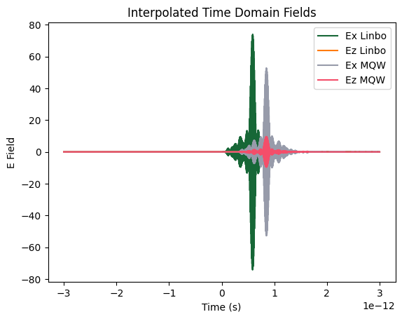
Get all previously simulated fields (at the center position) on one time axis:
dt = 0.2e-15  # time step in seconds
time = np.arange(-3000e-15, 3000e-15, dt)
time = time - time[time.size//2]  # ensure there is a proper 0 point

freqs = np.fft.fftfreq(len(time), time[1]-time[0])
ex_linbo3_td = np.interp(
    time, t_linbo-np.mean(t_linbo), etx_linbo, left=0, right=0)
ez_linbo3_td = np.interp(
    time, t_linbo-np.mean(t_linbo), etz_linbo, left=0, right=0)
ex_mqw_td = np.interp(
    time, t_mqw-np.mean(t_mqw), etx_mqw, left=0, right=0)
ez_mqw_td = np.interp(
    time, t_mqw-np.mean(t_mqw), etz_mqw, left=0, right=0)

plt.plot(time, ex_linbo3_td)
plt.plot(time, ez_linbo3_td)
plt.plot(time, ex_mqw_td)
plt.plot(time, ez_mqw_td)
plt.xlabel('Time (s)')
plt.ylabel('E Field')
plt.title('Interpolated Time Domain Fields')
plt.legend(['Ex Linbo', 'Ez Linbo', 'Ex MQW', 'Ez MQW'])
plt.show()
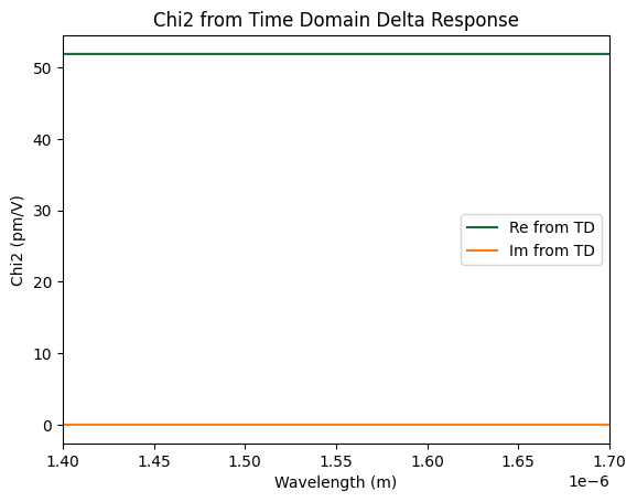
Define the time domain response function for linbo and calculate the spectral response as a consequence:
# assume a delta function nonlinear response in time for linbo3
# assume independent responses for both photons
# define delay variables to avoid confusion in convolution
tau1 = time
tau2 = time
decay1 = np.zeros_like(tau1)
decay2 = np.zeros_like(tau2)
decay1[decay1.size//2] = 1  # very broad response (delta in time)
decay2[decay2.size//2] = 1  # very broad response (delta in time)
decay1 = decay1 / np.sum(decay1) / dt
decay2 = decay2 / np.sum(decay2) / dt

# calculate the chi2 in frequency domain from the time domain response
# via convolution, this is not necessary but to check the magnitude
# and shape of the response
chi_2_linbo3_fd_from_td = np.zeros_like(freqs, dtype=complex)
for idx, f in enumerate(tqdm(freqs)):
    chi_2_linbo3_fd_from_td[idx] = chi_2_linbo3 * np.sum(
        np.sum(decay1 * np.exp(1j*2*np.pi*f*tau1))
        * decay2 * np.exp(1j*2*np.pi*f*tau2))*dt*dt

# plot
wls_out = c / (freqs+1)
plt.plot(wls_out, np.real(chi_2_linbo3_fd_from_td))
plt.plot(wls_out, np.imag(chi_2_linbo3_fd_from_td))
plt.xlim([1400e-9, 1700e-9])
plt.xlabel('Wavelength (m)')
plt.ylabel('Chi2 (pm/V)')
plt.legend(['Re from TD', 'Im from TD'])
plt.title('Chi2 from Time Domain Delta Response')
plt.show()
100%|██████████| 30001/30001 [00:20<00:00, 1468.83it/s]
Calculate the SHG generated by the incident fields via convolution in the time domain; independent photons allow us to convolve separately:
res2 = np.convolve(
        decay2,
        ex_linbo3_td, 'same')*dt
res1 = np.convolve(
    decay1,
    ex_linbo3_td, 'same')*dt
e_2f_linbo3_td = chi_2_linbo3*res1*res2
e_2f_linbo3_td = e_2f_linbo3_td*effective_length_linbo3

e_2f_linbo3_fd = (
    np.fft.fft(np.fft.fftshift(e_2f_linbo3_td))
    * np.size(e_2f_linbo3_td))
# filter irrelevant/unphysical frequency components
e_2f_linbo3_fd[np.abs(np.abs(freqs)-0.39e15) > 0.1e15] = 0

# should be n1*n2*n3 but the n1 and n2 are
# already taken into account in the fields by tidy3d
# there is a correction factor of 0.75 (relative, not absolute) here,
# which is calculated from the propagation outside of the material
# (done similarly like the propagation inside the material)
intensity_2f_linbo3_fd = np.abs(e_2f_linbo3_fd)**2 / n_linbo3_shg / 0.75
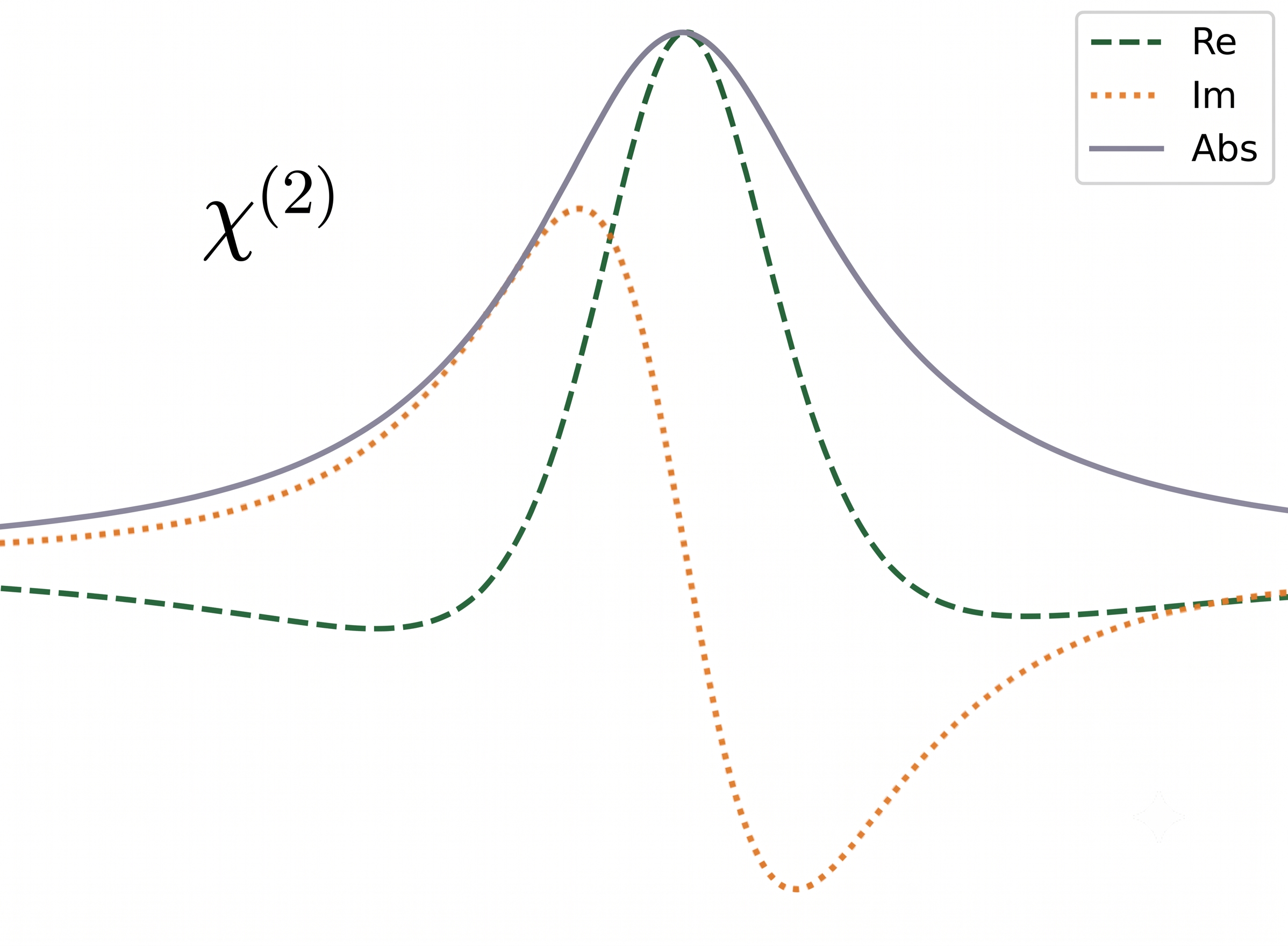
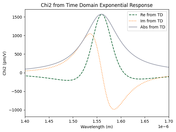
Define the time domain response function for the mqw and calculate the spectral response as a consequence:
# assume an exponentially decaying oscillator response in time for the mqw
# assume independent responses for both photons
amplitude_mqw = 1562  # pm/V, peak value
# define delay variables to avoid confusion in convolution
tau1 = time
tau2 = time
decay1 = np.exp(-tau1 / 30e-15)
decay2 = np.exp(-tau2 / 30e-15)
decay1[tau1 < 0] = 0.  # ensure causality
decay2[tau2 < 0] = 0.  # ensure causality
decay1 = decay1 / np.sum(decay1) / dt
decay2 = decay2 / np.sum(decay2) / dt
decay1 = decay1 * 2 * np.cos(2 * np.pi * 0.1923e15 * tau1)  # MQW resonance
decay2 = decay2 * 2 * np.cos(2 * np.pi * 0.1923e15 * tau2)  # MQW resonance

# calculate the chi2 in frequency domain from the time domain response
# via convolution, this is not necessary but to check the magnitude
# and shape of the response
chi_2_mqw_fd_from_td = np.zeros_like(freqs, dtype=complex)
for idx, f in enumerate(tqdm(freqs)):
    chi_2_mqw_fd_from_td[idx] = amplitude_mqw * np.sum(
        np.sum(decay1 * np.exp(1j*2*np.pi*f*tau1))
        * decay2 * np.exp(1j*2*np.pi*f*tau2))*dt*dt

plt.plot(wls_out, np.real(chi_2_mqw_fd_from_td), '--')
plt.plot(wls_out, np.imag(chi_2_mqw_fd_from_td), ':')
plt.plot(wls_out, np.abs(chi_2_mqw_fd_from_td), '-')
plt.xlabel('Wavelength (m)')
plt.ylabel('Chi2 (pm/V)')
plt.title('Chi2 from Time Domain Exponential Response')
plt.legend(['Re from TD', 'Im from TD', 'Abs from TD'])
plt.xlim([1400e-9, 1700e-9])
plt.show()
100%|██████████| 30001/30001 [00:20<00:00, 1447.59it/s]
Calculate the SHG generated by the incident fields via convolution in the time domain; independent photons allow us to convolve separately:
res2 = np.convolve(
    decay2, ez_mqw_td, 'same')*dt
res1 = np.convolve(
    decay1, ex_mqw_td, 'same')*dt
e_2f_mqw_td = amplitude_mqw*res1*res2
e_2f_mqw_td = e_2f_mqw_td*effective_length_mqw

e_2f_mqw_fd = np.fft.fft(np.fft.fftshift(e_2f_mqw_td)) * np.size(e_2f_mqw_td)

# should be n1*n2*n3 but the n1 and n2 are
# already taken into account in the fields by tidy3d
# there is a correction factor of 1.4 (relative, not absolute) here,
# which is calculated from the propagation outside of the material
# (done similarly like the propagation inside the material)
intensity_2f_mqw_fd = np.abs(e_2f_mqw_fd)**2 / n_mqw_shg / 1.4
Scale and plot the results to compare with the measurements:
intensity_2f_linbo3_wls = intensity_2f_linbo3_fd/(c/(freqs+1)**2)
intensity_2f_mqw_wls = intensity_2f_mqw_fd/(c/(freqs+1)**2)

# only count the relevant region around the SHG peak for scaling
mask_td = (wls_out > 720e-9) & (wls_out < 820e-9)
mask = (wls_shg > 720e-9) & (wls_shg < 820e-9)

scale = (
    -np.trapezoid(intensity_2f_linbo3_wls[mask_td], wls_out[mask_td])
    / np.trapezoid(intensity_linbo3_meas[mask], wls_shg[mask]))

plt.plot(
    wls_out, intensity_2f_linbo3_wls, 'b-',
    label='LiNbO3, td sim, ' + str(chi_2_linbo3) + ' pm/V')
plt.plot(
    wls_out, intensity_2f_mqw_wls, 'r-',
    label='MQW, td sim, ' + str(amplitude_mqw) + ' pm/V')
plt.plot(wls_shg, intensity_linbo3_meas*scale, 'b--', label='LiNbO3, exp')
plt.plot(wls_shg, intensity_mqw_meas*scale, 'r--', label='MQW, exp')
plt.legend()
plt.xlim([720e-9, 820e-9])
plt.xlabel('Wavelength (m)')
plt.ylabel('Intensity')
plt.show()

print(
    'integral comparison linbo3 (should be 1 if everything is correct): ',
    -np.trapezoid(intensity_2f_linbo3_wls[mask_td], wls_out[mask_td])
    / np.trapezoid(intensity_linbo3_meas[mask]*scale, wls_shg[mask]))

print(
    'integral comparison mqw (should be 1 if everything is correct): ',
    -np.trapezoid(intensity_2f_mqw_wls[mask_td], wls_out[mask_td])
    / np.trapezoid(intensity_mqw_meas[mask]*scale, wls_shg[mask]))
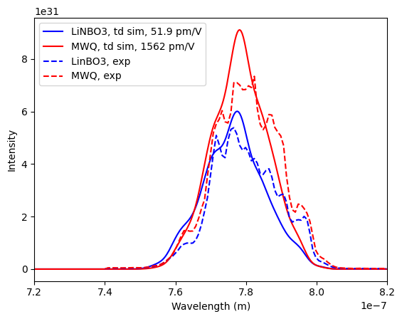
integral comparison linbo3 (should be 1 if everything is correct):  0.9999999999999999
integral comparison mwq (should be 1 if everything is correct):  0.9955879835234879



 TERMS & CONDITIONS


 How the process works:
 Try this real URL to see an example: