Authors: Judson D. Ryckman & Matthew Panipinto, Clemson University

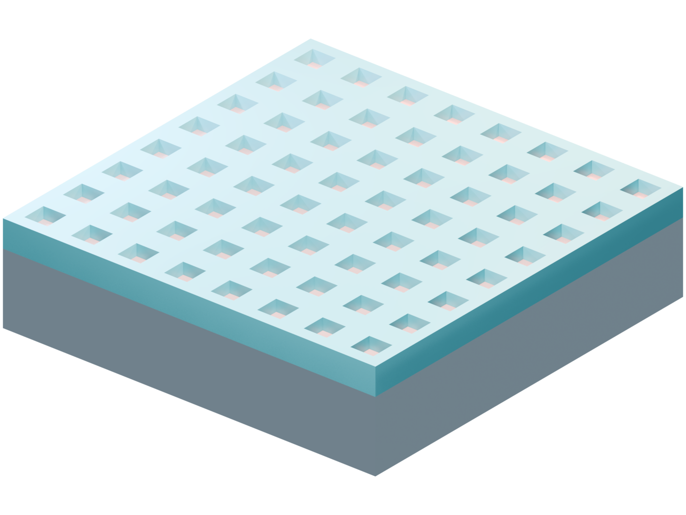
This notebook integrates the 2-component Bruggeman effective medium model with Tidy3D using the FastDispersionFitter plugin. It computes the dispersion of porous titania in both its uncompressed and compressed states, fits them to PoleResidue models, and runs the metasurface simulation.

[1]:

import os
import csv
import numpy as np
import matplotlib.pyplot as plt
import tidy3d as td
import tidy3d.web as web
from tidy3d.plugins.dispersion import FastDispersionFitter

Simulation Layout & Symmetry Breaking¶

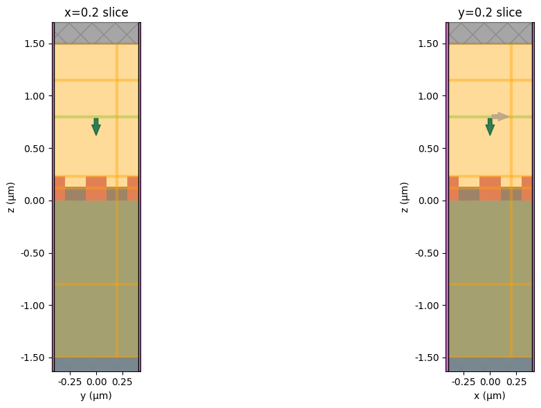
The simulation layout is constructed with periodic boundary conditions representing a unit cell that spans 2 periods in size (a 2x2 pillar quadrimer structure). This allows for symmetry breaking of the quadrimer by using the displacement parameter dX. Non-zero values of dX break the structural symmetry of the unit cell, enabling the excitation of quasi-bound states in the continuum (qBIC) modes. By default, dX = 0.0 preserves standard lattice symmetry, simulating a conventional guided mode resonance (GMR) metasurface.

[2]:

# Simulation parameters (microns)
period = 0.4
wl_min = 0.4
wl_max = 0.7
size_z = 3
slab_thick = 0.23
dX = 0.0  # Non-zero for qBIC
p0 = 0.565  # Uncompressed porosity
imprint_frac = 0.4345  # Film compression C
theta = 0
phi = 0
pol_angle = 0
# Substrate is loaded from Tidy3D's material library (BK7)
courant = 0.95  # Courant stability factor
shutoff = 1e-7  # Simulation shutoff threshold
run_time = 8e-12  # Simulation run time (seconds)
monitor_wls = np.linspace(0.4, 0.7, 151)  # Wavelengths for field monitors


# Load skeleton data
def load_anatase_skeleton(filepath="misc/Jolivet-anatase.csv"):
    if not os.path.exists(filepath):
        raise FileNotFoundError(f"Anatase skeleton file not found: {filepath}")
    wl_list = []
    n_list = []
    with open(filepath, mode="r", encoding="utf-8") as f:
        reader = csv.reader(f)
        next(reader)
        for row in reader:
            if not row or row[0].strip() == "" or "wl" in row[0]:
                break
            wl_list.append(float(row[0]))
            n_list.append(float(row[1]))
    return np.array(wl_list), np.array(n_list)


wl_sk, n_sk = load_anatase_skeleton("misc/Jolivet-anatase.csv")


# Bruggeman solver
def solve_bruggeman(p, n_skeleton):
    eps_sk = n_skeleton**2
    A = 2.0
    B = (3.0 * p - 2.0) * eps_sk + 1.0 - 3.0 * p
    C_val = -eps_sk
    y = (-B + np.sqrt(B**2 - 4.0 * A * C_val)) / (2.0 * A)
    return np.sqrt(y)


# Define porosities
c_comp = imprint_frac  # Film compression
p_comp = (p0 - c_comp) / (1.0 - c_comp)  # Compressed porosity

# Grid of wavelengths for fitting (0.4 to 0.7 um)
wl_fit = np.linspace(wl_min, wl_max, 201)
n_sk_fit = np.interp(wl_fit, wl_sk, n_sk)

# Calculate dispersion index curves
n_uncompressed = solve_bruggeman(p0, n_sk_fit)
n_compressed = solve_bruggeman(p_comp, n_sk_fit)
k_fit = np.zeros_like(wl_fit)  # assume negligible absorption

print(f"Fitting uncompressed pTiO2 (p={p0:.2f}) using FastDispersionFitter...")
fitter_un = FastDispersionFitter(wvl_um=wl_fit, n_data=n_uncompressed, k_data=k_fit)
porous_titania_uncompressed, rms_un = fitter_un.fit(
    min_num_poles=2, max_num_poles=4, tolerance_rms=1e-3
)
print(f"  Uncompressed Fit RMS: {rms_un:.2e}")

print(
    f"Fitting compressed pTiO2 (p={p_comp:.4f}, C={c_comp:.2f}) using FastDispersionFitter..."
)
fitter_co = FastDispersionFitter(wvl_um=wl_fit, n_data=n_compressed, k_data=k_fit)
porous_titania_compressed, rms_co = fitter_co.fit(
    min_num_poles=2, max_num_poles=4, tolerance_rms=1e-3
)
print(f"  Compressed Fit RMS: {rms_co:.2e}")

Output()

Fitting uncompressed pTiO2 (p=0.56) using FastDispersionFitter...

Output()

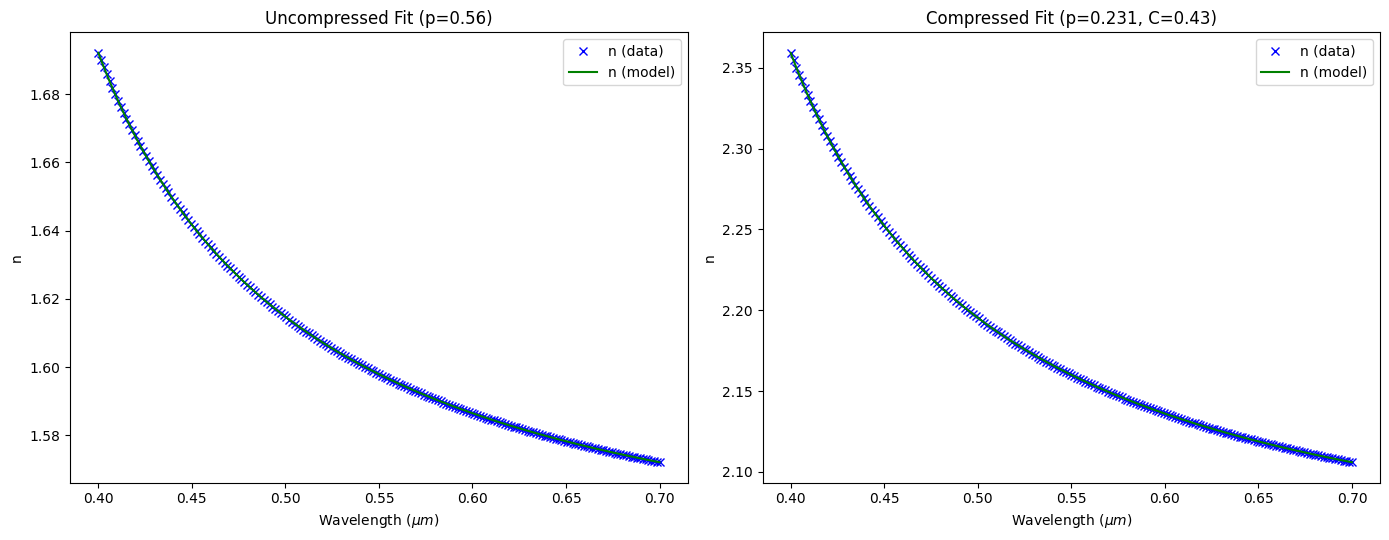
  Uncompressed Fit RMS: 4.49e-07
Fitting compressed pTiO2 (p=0.2308, C=0.43) using FastDispersionFitter...

  Compressed Fit RMS: 4.46e-06

Verify Dispersion Fitting Quality¶

Plot the calculated Bruggeman refractive index data points and the fitted curves to check for accuracy.

[3]:

fig, (ax1, ax2) = plt.subplots(1, 2, figsize=(14, 5.5))
fitter_un.plot(porous_titania_uncompressed, ax=ax1)
ax1.set_title(f"Uncompressed Fit (p={p0:.2f})")
fitter_co.plot(porous_titania_compressed, ax=ax2)
ax2.set_title(f"Compressed Fit (p={p_comp:.3f}, C={c_comp:.2f})")
plt.tight_layout()
plt.show()

No description has been provided for this image

Create Tidy3D Simulation Setup¶

Define background medium, source, monitors, and the metasurface structure using our dynamic materials.

[4]:

air = td.Medium(
    name="air",
    viz_spec=td.VisualizationSpec(facecolor="#a6a6a6", edgecolor="#000000", alpha=0.31),
)

plane_wave = td.PlaneWave(
    name="plane_wave",
    center=[0, 0, size_z / 2 - wl_max],
    size=[td.inf, td.inf, 0],
    source_time=td.GaussianPulse(
        freq0=615645226250000,
        fwidth=481809307500000,
    ),
    direction="-",
    angle_theta=theta * np.pi / 180,
    angle_phi=phi * np.pi / 180,
    pol_angle=pol_angle * np.pi / 180,
    angular_spec=td.FixedInPlaneKSpec(),
)

Reflection = td.FluxMonitor(
    name="Reflection",
    center=[0, 0, size_z / 2 - wl_max / 2],
    size=[10, 10, 0],
    freqs=td.C_0 / np.linspace(0.35, 0.8, 1751),
    normal_dir="+",
)

field_XZ = td.FieldMonitor(
    name="field_XZ",
    center=[0, period / 2, 0],
    size=[10, 0, size_z],
    freqs=td.C_0 / monitor_wls,
)

field_YZ = td.FieldMonitor(
    name="field_YZ",
    center=[period / 2, 0, 0],
    size=[0, 10, size_z],
    freqs=td.C_0 / monitor_wls,
)

permittivitymonitor = td.PermittivityMonitor(
    name="permittivitymonitor",
    center=[0, 0, slab_thick],
    size=[5, 5, 0],
    freqs=td.C_0 / 0.575,
    apodization=td.ApodizationSpec(),
)

field_XY = td.FieldMonitor(
    name="field_XY",
    center=[0, 0, slab_thick / 2],
    size=[10, 10, 0],
    freqs=td.C_0 / monitor_wls,
)

Transmission = td.FluxMonitor(
    name="Transmission",
    center=[0, 0, -size_z / 2 + wl_max],
    size=[10, 10, 0],
    freqs=td.C_0 / np.linspace(0.35, 0.8, 1751),
    normal_dir="-",
)

substrate_medium = td.material_library["BK7"].medium

substrate = td.Structure(
    name="substrate",
    geometry=td.Box(center=[0, 0, -500], size=[2000, 2000, 1000]),
    medium=substrate_medium,
)

core_slab = td.Structure(
    name="core_slab",
    geometry=td.Box(center=[0, 0, slab_thick / 2], size=[5, 5, slab_thick]),
    medium=porous_titania_uncompressed,
)

core_pillar_air = td.Structure(
    name="core_pillar_air",
    geometry=td.Box(
        center=[-period / 2 - dX, -period / 2 - dX, slab_thick / 2],
        size=[period / 2, period / 2, slab_thick],
    ),
    medium=air,
)

core_pillar_copy_air = td.Structure(
    name="core_pillar_copy_air",
    geometry=td.Box(
        center=[period / 2 + dX, period / 2 + dX, slab_thick / 2],
        size=[period / 2, period / 2, slab_thick],
    ),
    medium=air,
)

core_pillar_copy_Copy_air = td.Structure(
    name="core_pillar_copy_Copy_air",
    geometry=td.Box(
        center=[period / 2 + dX, -period / 2 - dX, slab_thick / 2],
        size=[period / 2, period / 2, slab_thick],
    ),
    medium=air,
)

core_pillar_Copy_Copy_air = td.Structure(
    name="core_pillar_Copy_Copy_air",
    geometry=td.Box(
        center=[-period / 2 - dX, +period / 2 + dX, slab_thick / 2],
        size=[period / 2, period / 2, slab_thick],
    ),
    medium=air,
)

core_pillar = td.Structure(
    name="core_pillar",
    geometry=td.Box(
        center=[
            -period / 2 - dX,
            -period / 2 - dX,
            (1 - imprint_frac) * slab_thick / 2,
        ],
        size=[period / 2, period / 2, (1 - imprint_frac) * slab_thick],
    ),
    medium=porous_titania_compressed,
)

core_pillar_copy = td.Structure(
    name="core_pillar_copy",
    geometry=td.Box(
        center=[period / 2 + dX, period / 2 + dX, (1 - imprint_frac) * slab_thick / 2],
        size=[period / 2, period / 2, (1 - imprint_frac) * slab_thick],
    ),
    medium=porous_titania_compressed,
)

core_pillar_copy_Copy = td.Structure(
    name="core_pillar_copy_Copy",
    geometry=td.Box(
        center=[period / 2 + dX, -period / 2 - dX, (1 - imprint_frac) * slab_thick / 2],
        size=[period / 2, period / 2, (1 - imprint_frac) * slab_thick],
    ),
    medium=porous_titania_compressed,
)

core_pillar_Copy = td.Structure(
    name="core_pillar_Copy",
    geometry=td.Box(
        center=[
            -period / 2 - dX,
            +period / 2 + dX,
            (1 - imprint_frac) * slab_thick / 2,
        ],
        size=[period / 2, period / 2, (1 - imprint_frac) * slab_thick],
    ),
    medium=porous_titania_compressed,
)

sim = td.Simulation(
    size=[0.8, 0.8, 3],
    boundary_spec=td.BoundarySpec(
        x=td.Boundary(
            plus=td.BlochBoundary(bloch_vec=0), minus=td.BlochBoundary(bloch_vec=0)
        ),
        y=td.Boundary(
            plus=td.BlochBoundary(bloch_vec=0), minus=td.BlochBoundary(bloch_vec=0)
        ),
        z=td.Boundary(
            plus=td.PML(
                parameters=td.PMLParams(
                    kappa_min=1, kappa_max=3, alpha_order=1, alpha_max=0
                )
            ),
            minus=td.PML(
                parameters=td.PMLParams(
                    kappa_min=1, kappa_max=3, alpha_order=1, alpha_max=0
                )
            ),
        ),
    ),
    grid_spec=td.GridSpec.auto(wavelength=wl_min, min_steps_per_wvl=24),
    subpixel=td.SubpixelSpec(
        dielectric=td.PolarizedAveraging(),
        metal=td.Staircasing(),
        pec=td.PECConformal(),
    ),
    courant=courant,
    shutoff=shutoff,
    run_time=run_time,
    medium=air,
    sources=[plane_wave],
    monitors=[
        Reflection,
        field_XZ,
        field_YZ,
        permittivitymonitor,
        field_XY,
        Transmission,
    ],
    structures=[
        substrate,
        core_slab,
        core_pillar_air,
        core_pillar_copy_air,
        core_pillar_copy_Copy_air,
        core_pillar_Copy_Copy_air,
        core_pillar,
        core_pillar_copy,
        core_pillar_copy_Copy,
        core_pillar_Copy,
    ],
)

Visualize 2D Slices of Device Geometry¶

Plot the $x=0.2$ and $y=0.2$ cross sections to verify the structure definition before submitting to Tidy3D.

[5]:

fig, (ax1, ax2) = plt.subplots(1, 2, figsize=(15, 6))
sim.plot(x=period / 2, ax=ax1)
ax1.set_title(f"x={period / 2} slice")
sim.plot(y=period / 2, ax=ax2)
ax2.set_title(f"y={period / 2} slice")
plt.tight_layout()
plt.show()

Run the Simulation on Tidy3D Web Server¶

[6]:

sim_data = web.run(
    sim, task_name="pTiO2_Quadrimer_Dispersive_FDTD", path="./data/sim_data.hdf5"
)

14:38:47 KST Loading simulation from local cache. View cached task using web UI 
             at                                                                 
             'https://tidy3d.simulation.cloud/workbench?taskId=fdve-56451b30-d12
             d-4b1b-b9d9-4aae0bc36d6b'.

             WARNING: Simulation final field decay value of 0.000124 is greater 
             than the simulation shutoff threshold of 1e-07. Consider running   
             the simulation again with a larger 'run_time' duration for more    
             accurate results.

Data Analysis and Plotting¶

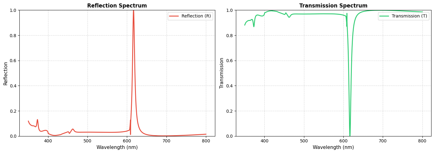
Plot the reflection and transmission spectra extracted from the flux monitors.

[7]:

# Extract flux from monitors
refl_flux = sim_data["Reflection"].flux
trans_flux = sim_data["Transmission"].flux

freqs = refl_flux.f.values
wl_nm = (td.C_0 / freqs) * 1e3  # convert to nm

# Compute coefficients
R = np.abs(refl_flux.values)
T = np.abs(trans_flux.values)

# Plot Reflection and Transmission on separate subplots
fig, (ax1, ax2) = plt.subplots(1, 2, figsize=(14, 5))

# Reflection plot
ax1.plot(wl_nm, R, label="Reflection (R)", color="#e74c3c", linewidth=2)
ax1.set_xlabel("Wavelength (nm)", fontsize=11)
ax1.set_ylabel("Reflection", fontsize=11)
ax1.set_title("Reflection Spectrum", fontsize=12, fontweight="bold")
ax1.set_ylim(0.0, 1.0)
ax1.grid(True, linestyle="--", alpha=0.5)
ax1.legend(fontsize=10)

# Transmission plot
ax2.plot(wl_nm, T, label="Transmission (T)", color="#2ecc71", linewidth=2)
ax2.set_xlabel("Wavelength (nm)", fontsize=11)
ax2.set_ylabel("Transmission", fontsize=11)
ax2.set_title("Transmission Spectrum", fontsize=12, fontweight="bold")
ax2.set_ylim(0.0, 1.0)
ax2.grid(True, linestyle="--", alpha=0.5)
ax2.legend(fontsize=10)

plt.tight_layout()
plt.show()

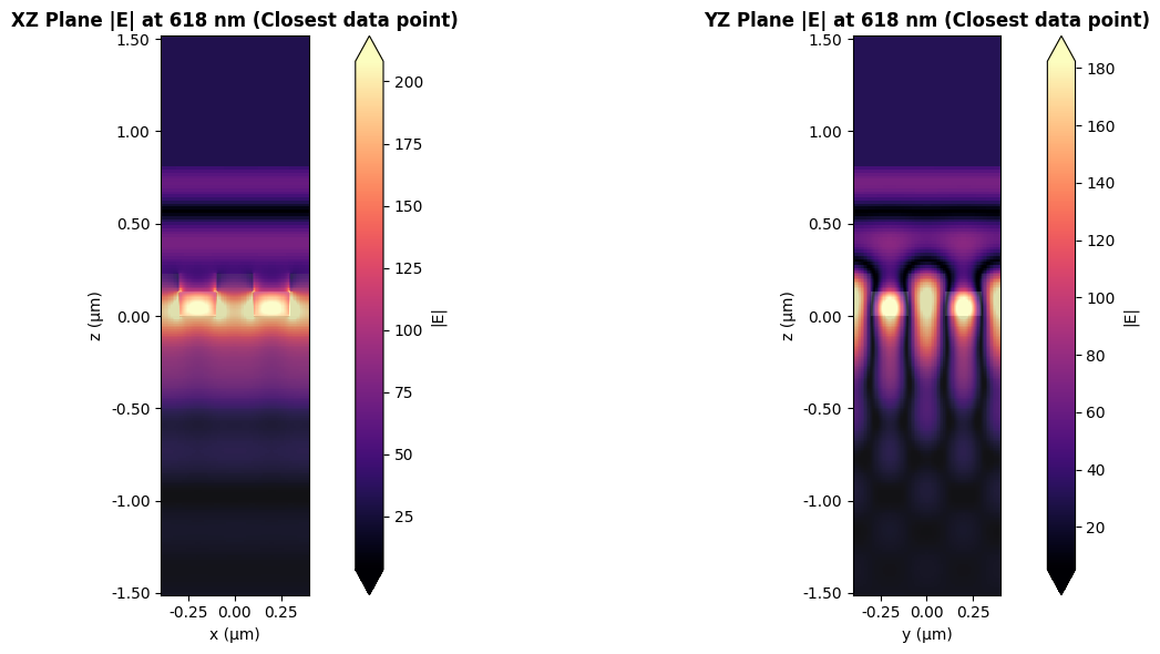
Plot Electric Field Distribution¶

Visualize the electric field profile $|E|$ in the $x-z$ plane at a specific wavelength, such as at a resonance point or a chosen wavelength.

[8]:

# Set wavelength of interest (e.g. 618 nm)
wvl_interest = 0.618  # um

# Find closest frequency using the global monitor_wls array (pSiGMR style)
idx = np.abs(monitor_wls - wvl_interest).argmin()
freq_closest = td.C_0 / monitor_wls[idx]
wvl_closest_nm = int(monitor_wls[idx] * 1000)

fig, (ax1, ax2) = plt.subplots(1, 2, figsize=(15, 6))
# Use positional arguments to avoid TypeError
sim_data.plot_field("field_XZ", "E", "abs", f=freq_closest, ax=ax1)
ax1.set_title(
    f"XZ Plane |E| at {wvl_closest_nm} nm (Closest data point)",
    fontsize=12,
    fontweight="bold",
)

sim_data.plot_field("field_YZ", "E", "abs", f=freq_closest, ax=ax2)
ax2.set_title(
    f"YZ Plane |E| at {wvl_closest_nm} nm (Closest data point)",
    fontsize=12,
    fontweight="bold",
)

plt.tight_layout()
plt.show()

TIDY3D
LEARNING CENTER

pTiO2 dispersive simulation with Bruggeman model¶

Simulation Layout & Symmetry Breaking¶

Verify Dispersion Fitting Quality¶

Create Tidy3D Simulation Setup¶

Visualize 2D Slices of Device Geometry¶

Run the Simulation on Tidy3D Web Server¶

Data Analysis and Plotting¶

Plot Electric Field Distribution¶

More Notebooks

TIDY3D LEARNING CENTER

pTiO2 dispersive simulation with Bruggeman model¶

Simulation Layout & Symmetry Breaking¶

Verify Dispersion Fitting Quality¶

Create Tidy3D Simulation Setup¶

Visualize 2D Slices of Device Geometry¶

Run the Simulation on Tidy3D Web Server¶

Data Analysis and Plotting¶

Plot Electric Field Distribution¶

More Notebooks

Cookie preferences

Privacy choices

TIDY3D
LEARNING CENTER