





Authors: Anna Kulter, Marcus Ossiander, Graz University of Technology
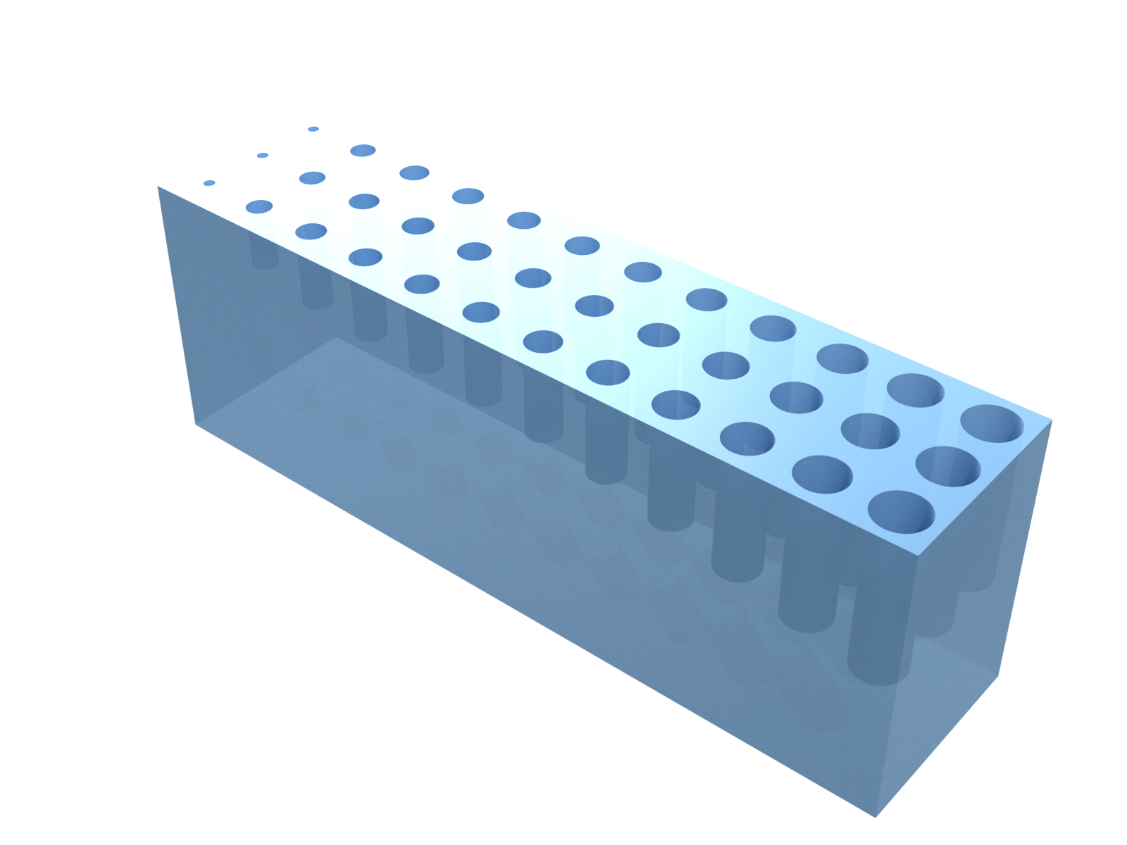
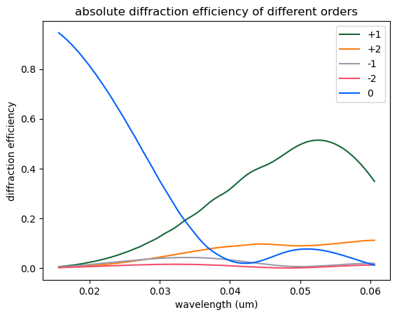
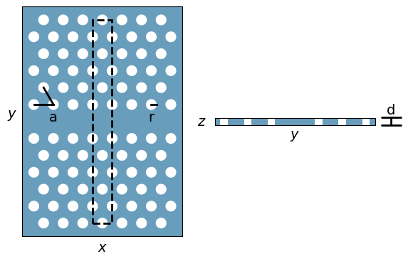
Example script using Tidy3D to simulate energy-resolved diffraction by a metagrating in the extreme ultraviolet. The metagrating is made of a silicon membrane with vacuum holes. The hole diameter sets the local transmission phase, and a phase ramp that repeats every 12 holes blazes the grating towards one diffraction order. The silicon material is fitted to experimental data using the FastDispersionFitter plugin. The diffraction efficiency of the different orders is plotted as a function of wavelength.
The device and its characterization are described in Anna Kulter, Tiago Regio Crispim, Lorenz Weiss, Alexander Sagar Grossek, David J. Grafinger, Zsuzsanna Pápa, Judit Budai, Lázár Tóth, Péter Dombi, Rodolfo Previdi, Harald Plank, Andreas Hohenau, Martin Schultze, and Marcus Ossiander, "Transmissive extreme ultraviolet metagrating", arXiv:2607.06174 (2026). DOI: 10.48550/arXiv.2607.06174. The data files are available in this repository.
import numpy as np
import matplotlib.pyplot as plt

import tidy3d as td
import tidy3d.web as web
from tidy3d.plugins.dispersion import AdvancedFastFitterParam
from tidy3d.plugins.dispersion import FastDispersionFitter
Silicon Material Model
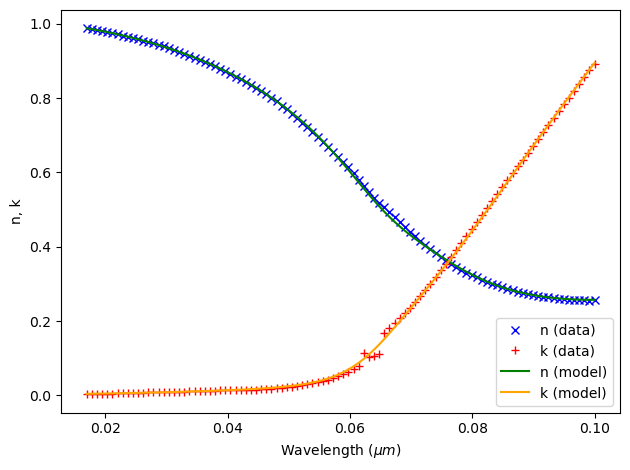
First create a dispersive material describing silicon in the extreme ultraviolet from published $n$, $k$ data (Handbook of Optical Constants of Solids, Ed. by Edward D. Palik, Academic Press, Inc., 1985):
n_data = np.array(
      [0.9879997 , 0.98548329, 0.98296484, 0.97993533, 0.97729243,
       0.97522844, 0.97187035, 0.96851581, 0.96516665, 0.96181891,
       0.95846265, 0.95510131, 0.95169247, 0.94750055, 0.94331637,
       0.93911683, 0.93407661, 0.92871212, 0.92433052, 0.91849045,
       0.91414237, 0.90875595, 0.90289607, 0.8972943 , 0.89201133,
       0.88528947, 0.87860733, 0.87187492, 0.86469118, 0.85779876,
       0.85147876, 0.84313829, 0.83551906, 0.82733101, 0.81897704,
       0.81024036, 0.80097632, 0.79169783, 0.78002466, 0.76958251,
       0.75844979, 0.74641808, 0.73389504, 0.72127624, 0.70776345,
       0.69513171, 0.68196387, 0.66853307, 0.65534885, 0.64246833,
       0.62851169, 0.6142874 , 0.59796305, 0.57970135, 0.56339033,
       0.54763839, 0.5315947 , 0.51680252, 0.50785563, 0.49406955,
       0.48037768, 0.46686698, 0.45342287, 0.44045951, 0.42865372,
       0.41651544, 0.40489567, 0.39392987, 0.38263384, 0.37221311,
       0.36331693, 0.35468624, 0.34624684, 0.33802907, 0.33045665,
       0.32385312, 0.31743246, 0.31129183, 0.30572282, 0.30069342,
       0.29590888, 0.29128076, 0.28686106, 0.28294886, 0.27937509,
       0.27613726, 0.27297326, 0.26984923, 0.26753752, 0.26552905,
       0.26357446, 0.26163913, 0.26006383, 0.25866606, 0.25753061,
       0.25663394, 0.25587369, 0.2554426 , 0.25501151, 0.25540316])

k_data = np.array(
      [0.00254004, 0.00290073, 0.00328206, 0.00368808, 0.00410689,
       0.00453995, 0.00501718, 0.00546166, 0.00593375, 0.00642716,
       0.0069306 , 0.00742357, 0.00788383, 0.00834494, 0.00884204,
       0.00928832, 0.00970881, 0.01010303, 0.01036174, 0.01002803,
       0.01100298, 0.01154252, 0.01187737, 0.01218529, 0.01244943,
       0.01278553, 0.01311963, 0.01339219, 0.01364363, 0.01392579,
       0.01427606, 0.01469309, 0.01511561, 0.01560014, 0.0163023 ,
       0.01714179, 0.01805756, 0.01922806, 0.020312  , 0.02176262,
       0.0233786 , 0.02508147, 0.02697959, 0.02934928, 0.03213629,
       0.03539821, 0.03875903, 0.04252092, 0.04683876, 0.05163069,
       0.05737754, 0.0632346 , 0.07041663, 0.07825379, 0.11386598,
       0.10214226, 0.10531568, 0.11009219, 0.16850875, 0.18086868,
       0.19362232, 0.20713302, 0.22089255, 0.23644859, 0.25158808,
       0.26764608, 0.2841565 , 0.30102385, 0.31832792, 0.3362164 ,
       0.35383972, 0.37220595, 0.3911946 , 0.40968459, 0.42837572,
       0.44752595, 0.46614587, 0.4848837 , 0.50406585, 0.52281299,
       0.5413645 , 0.55987697, 0.57853199, 0.59753409, 0.6162078 ,
       0.63455554, 0.65316045, 0.6719046 , 0.69052799, 0.70910629,
       0.72754266, 0.74592827, 0.76448223, 0.78311919, 0.80162252,
       0.8200042 , 0.83830504, 0.85641082, 0.8745166 , 0.89233597])

wls_material_fit = np.array(
      [0.017     , 0.01783838, 0.01867677, 0.01951515, 0.02035354,
       0.02119192, 0.0220303 , 0.02286869, 0.02370707, 0.02454545,
       0.02538384, 0.02622222, 0.02706061, 0.02789899, 0.02873737,
       0.02957576, 0.03041414, 0.03125253, 0.03209091, 0.03292929,
       0.03376768, 0.03460606, 0.03544444, 0.03628283, 0.03712121,
       0.0379596 , 0.03879798, 0.03963636, 0.04047475, 0.04131313,
       0.04215152, 0.0429899 , 0.04382828, 0.04466667, 0.04550505,
       0.04634343, 0.04718182, 0.0480202 , 0.04885859, 0.04969697,
       0.05053535, 0.05137374, 0.05221212, 0.05305051, 0.05388889,
       0.05472727, 0.05556566, 0.05640404, 0.05724242, 0.05808081,
       0.05891919, 0.05975758, 0.06059596, 0.06143434, 0.06227273,
       0.06311111, 0.06394949, 0.06478788, 0.06562626, 0.06646465,
       0.06730303, 0.06814141, 0.0689798 , 0.06981818, 0.07065657,
       0.07149495, 0.07233333, 0.07317172, 0.0740101 , 0.07484848,
       0.07568687, 0.07652525, 0.07736364, 0.07820202, 0.0790404 ,
       0.07987879, 0.08071717, 0.08155556, 0.08239394, 0.08323232,
       0.08407071, 0.08490909, 0.08574747, 0.08658586, 0.08742424,
       0.08826263, 0.08910101, 0.08993939, 0.09077778, 0.09161616,
       0.09245455, 0.09329293, 0.09413131, 0.0949697 , 0.09580808,
       0.09664646, 0.09748485, 0.09832323, 0.09916162, 0.1       ])
fitter = FastDispersionFitter(
    wvl_um=wls_material_fit,
    n_data=n_data,
    k_data=k_data)

si_material, rms_error = fitter.fit(
    max_num_poles=2,
    advanced_param=AdvancedFastFitterParam(weights=(1, 1)),
    tolerance_rms=2e-2)

fitter.plot(si_material)
plt.show()

vacuum_material = td.Medium(name='Vacuum')
Output()
Simulation Setup
Create a blazed metagrating simulation by cutting holes (vacuum) in a silicon membrane. Each hole is a Cylinder and all of them are collected in a single GeometryGroup placed on top of the silicon Structure. A PlaneWave illuminates the membrane at normal incidence, the supercell is Periodic along x and y and terminated by PML along z, and a DiffractionMonitor behind the membrane records the transmitted orders:
def make_sim(
        ref, wl_min, wl_max, wls,
        supercell_size_x_um,
        supercell_size_y_um,
        xx_positions_um,
        yy_positions_um,
        pillar_widths_metasurface_um,
        pillar_thicknesses_metasurface_um,
        substrate_thickness_um):

    tx = supercell_size_x_um
    ty = supercell_size_y_um
    tz = wl_max + substrate_thickness_um + wl_max

    source = td.PlaneWave(
        name='planewave_0',
        center=[0, 0, wl_max/2],
        size=[np.inf, np.inf, 0],
        source_time=td.GaussianPulse(
            freq0=td.C_0 / (1/((1/wl_max + 1/wl_min)/2)),
            fwidth=td.C_0 / (1/((1/wl_max + 1/wl_min)/2))*0.95),
        direction='+',
        angle_theta=0,
        pol_angle=0/180*np.pi) # 0 # 90 # 45

    substrate = td.Structure(
        geometry=td.Box(
            center=[0, 0, wl_max + substrate_thickness_um/2],
            size=[np.inf, np.inf, substrate_thickness_um]),
        name='substrate',
        medium=si_material)

    if not ref:
        pillars = []
        for x_position_um, y_position_um, w, t in zip(
                xx_positions_um.flatten(),
                yy_positions_um.flatten(),
                pillar_widths_metasurface_um.flatten(),
                pillar_thicknesses_metasurface_um.flatten()
                ):

                pillars.append(
                     td.Cylinder(
                        center=[
                             x_position_um,
                             y_position_um,
                             wl_max + substrate_thickness_um - t/2],
                        radius=w / 2,
                        length=t))

        pillar_geometry_group = td.Structure(
            name='pillars',
            geometry=td.GeometryGroup(geometries=pillars),
            medium=vacuum_material)

        structures = [substrate, pillar_geometry_group]
    else:
        structures = [substrate]

    monitor_diffraction = td.DiffractionMonitor(
        name="diffraction_monitor",
        center=[0, 0, wl_max + substrate_thickness_um + wl_max/2],
        size=[td.inf, td.inf, 0],
        freqs=td.C_0 / wls,
        normal_dir="+")

    periodic_boundary_x = td.Boundary(
            plus=td.Periodic(), minus=td.Periodic())
    periodic_boundary_y = td.Boundary(
            plus=td.Periodic(), minus=td.Periodic())
    pml_boundary_z = td.Boundary(
        plus=td.PML(parameters=td.PMLParams(
            kappa_min=1, kappa_max=3, alpha_order=1, alpha_max=0)),
        minus=td.PML(parameters=td.PMLParams(
            kappa_min=1, kappa_max=3, alpha_order=1, alpha_max=0)))

    sim = td.Simulation(
        center=[0, 0, tz/2],
        size=[tx, ty, tz],
        boundary_spec=td.BoundarySpec(
            x=periodic_boundary_x,
            y=periodic_boundary_y,
            z=pml_boundary_z),
        grid_spec=td.GridSpec.auto(
            wavelength=wl_min,
            min_steps_per_wvl=14),
        run_time=0.1e-12,
        medium=vacuum_material,
        sources=[source],
        monitors=[monitor_diffraction],
        structures=structures,
        shutoff=0.001,
        subpixel=td.SubpixelSpec(
            dielectric=td.PolarizedAveraging(),
            metal=td.VolumetricAveraging()),
        symmetry=(0, 0, 0))

    return sim
Meta-Atom Library
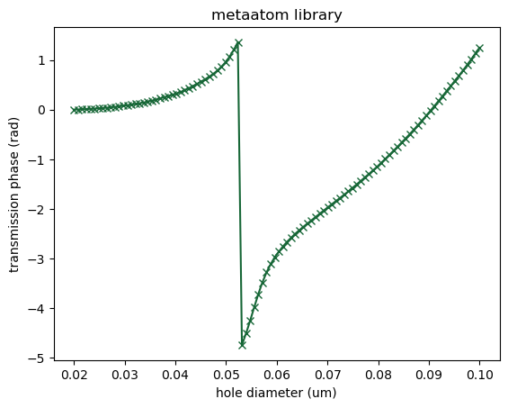
Load a meta-atom library (vacuum holes in a silicon membrane). The example library is calculated for a 500 nm thick membrane and a 120 nm unit cell size, and accounts for the experimentally determined etch depth:
unit_cell_size_um = 0.12
substrate_thickness_um = 0.5

pillar_diameters_um = np.array(
      [0.02      , 0.02080808, 0.02161616, 0.02242424, 0.02323232,
       0.0240404 , 0.02484848, 0.02565657, 0.02646465, 0.02727273,
       0.02808081, 0.02888889, 0.02969697, 0.03050505, 0.03131313,
       0.03212121, 0.03292929, 0.03373737, 0.03454545, 0.03535354,
       0.03616162, 0.0369697 , 0.03777778, 0.03858586, 0.03939394,
       0.04020202, 0.0410101 , 0.04181818, 0.04262626, 0.04343434,
       0.04424242, 0.04505051, 0.04585859, 0.04666667, 0.04747475,
       0.04828283, 0.04909091, 0.04989899, 0.05070707, 0.05151515,
       0.05232323, 0.05313131, 0.05393939, 0.05474747, 0.05555556,
       0.05636364, 0.05717172, 0.0579798 , 0.05878788, 0.05959596,
       0.06040404, 0.06121212, 0.0620202 , 0.06282828, 0.06363636,
       0.06444444, 0.06525253, 0.06606061, 0.06686869, 0.06767677,
       0.06848485, 0.06929293, 0.07010101, 0.07090909, 0.07171717,
       0.07252525, 0.07333333, 0.07414141, 0.07494949, 0.07575758,
       0.07656566, 0.07737374, 0.07818182, 0.0789899 , 0.07979798,
       0.08060606, 0.08141414, 0.08222222, 0.0830303 , 0.08383838,
       0.08464646, 0.08545455, 0.08626263, 0.08707071, 0.08787879,
       0.08868687, 0.08949495, 0.09030303, 0.09111111, 0.09191919,
       0.09272727, 0.09353535, 0.09434343, 0.09515152, 0.0959596 ,
       0.09676768, 0.09757576, 0.09838384, 0.09919192, 0.1       ])

phases_lib = np.array(
      [ 0.00000000e+00,  3.12240000e-03,  6.76600000e-03,  1.08514300e-02,
        1.54088800e-02,  2.01183300e-02,  2.54607500e-02,  3.16430700e-02,
        3.81748200e-02,  4.60674000e-02,  5.49236100e-02,  6.56567600e-02,
        7.66728600e-02,  8.78941600e-02,  1.00078430e-01,  1.12670290e-01,
        1.26157550e-01,  1.41471500e-01,  1.59340820e-01,  1.79885500e-01,
        2.01119680e-01,  2.24375070e-01,  2.48449370e-01,  2.71939710e-01,
        2.98275330e-01,  3.23753310e-01,  3.53709720e-01,  3.87695640e-01,
        4.29262410e-01,  4.71088190e-01,  5.16201810e-01,  5.63191160e-01,
        6.09283320e-01,  6.60282090e-01,  7.18991440e-01,  7.84058110e-01,
        8.63786430e-01,  9.52330390e-01,  1.06647228e+00,  1.19973448e+00,
        1.35518651e+00, -4.73587920e+00, -4.50742232e+00, -4.25075239e+00,
       -3.97899082e+00, -3.71351192e+00, -3.47820557e+00, -3.27782033e+00,
       -3.11415155e+00, -2.97343155e+00, -2.86076773e+00, -2.75778383e+00,
       -2.66228990e+00, -2.58052444e+00, -2.50072685e+00, -2.42916589e+00,
       -2.35912451e+00, -2.29299503e+00, -2.22788475e+00, -2.16194364e+00,
       -2.09523663e+00, -2.03020443e+00, -1.96552859e+00, -1.90200685e+00,
       -1.83850257e+00, -1.77531247e+00, -1.71131876e+00, -1.64476815e+00,
       -1.57617433e+00, -1.50670527e+00, -1.43677107e+00, -1.36705592e+00,
       -1.29659391e+00, -1.22473482e+00, -1.15063691e+00, -1.07349081e+00,
       -9.93682300e-01, -9.12419240e-01, -8.30358090e-01, -7.47334880e-01,
       -6.63119110e-01, -5.78500720e-01, -4.92011210e-01, -4.03155600e-01,
       -3.11873830e-01, -2.18728940e-01, -1.23100830e-01, -2.57986200e-02,
        7.27323600e-02,  1.72053620e-01,  2.72824490e-01,  3.74715630e-01,
        4.76156070e-01,  5.78348380e-01,  6.82310200e-01,  7.89112700e-01,
        8.99424290e-01,  1.01234094e+00,  1.12830711e+00,  1.24423828e+00])

# experimental etch depth
pillar_thicknesses_lib_um = pillar_diameters_um*4-0.07

plt.plot(pillar_diameters_um, phases_lib, 'x-')
plt.xlabel('hole diameter (um)')
plt.ylabel('transmission phase (rad)')
plt.title('metaatom library')
plt.show()
Blazed Phase Profile
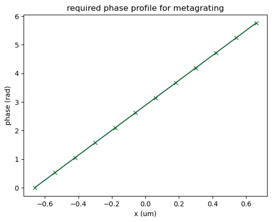
Calculate the blazed metagrating phase: a $2\pi$ phase shift every 12 holes along x, then repeat.
no_pillars_x = 12
no_pillars_y = 1
supercell_size_x_um = unit_cell_size_um*no_pillars_x
supercell_size_y_um = unit_cell_size_um*no_pillars_y

x_positions_um = (
    np.arange(0.5, no_pillars_x+0.5)*unit_cell_size_um
    - supercell_size_x_um/2)
y_positions_um = np.arange(0, 1)

xx_positions_um, yy_positions_um = np.meshgrid(x_positions_um, y_positions_um)

phase_profile = (
    2*np.pi/(unit_cell_size_um*12) * (xx_positions_um-np.min(x_positions_um)))
phase_profile = np.mod(phase_profile, 2*np.pi)

plt.plot(x_positions_um, phase_profile[0, :], 'x-')
plt.xlabel('x (um)')
plt.ylabel('phase (rad)')
plt.title('required phase profile for metagrating')
plt.show()
Match the required phase shift and the hole diameters to assemble the metagrating layout:
pillar_indices = np.zeros_like(xx_positions_um, dtype=int)
for i in range(xx_positions_um.shape[0]):
    for j in range(xx_positions_um.shape[1]):
        phase_diffs = np.mod(phases_lib - phase_profile[i, j], 2*np.pi)
        phase_diffs[phase_diffs > np.pi] = (
            phase_diffs[phase_diffs > np.pi] - 2*np.pi)
        pillar_indices[i, j] = np.argmin(np.abs(phase_diffs))
pillar_widths_metasurface_um = pillar_diameters_um[pillar_indices]
pillar_thicknesses_metasurface_um = pillar_thicknesses_lib_um[pillar_indices]

# roll for a prettier plot, no physical difference due to periodic boundaries
pillar_widths_metasurface_um = pillar_widths_metasurface_um
pillar_thicknesses_metasurface_um = pillar_thicknesses_metasurface_um

plt.plot(x_positions_um, pillar_widths_metasurface_um[0, :])
plt.xlabel('x (um)')
plt.ylabel('pillar width (um)')
plt.title('required pillar width distribution for metagrating')
plt.show()
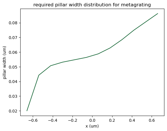
Metagrating Simulation
Assemble the supercell simulation over the target wavelength range:
tidy3d_folder = 'euv_metagrating'
ref_bool = False
wl_min = 1.03/66
wl_max = 1.03/17
wls = np.linspace(wl_min, wl_max, 200)
sim = make_sim(
        ref_bool, wl_min, wl_max, wls,
        supercell_size_x_um,
        supercell_size_y_um,
        xx_positions_um,
        yy_positions_um,
        pillar_widths_metasurface_um,
        pillar_thicknesses_metasurface_um,
        substrate_thickness_um)
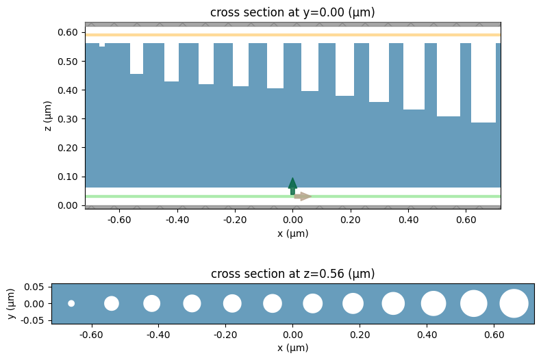
The xz cross section shows the etch depth of every hole, and the xy cut taken just below the top surface shows how the hole diameter grows along the supercell:
fig, (ax1, ax2) = plt.subplots(2, 1, figsize=(8, 6), tight_layout=True)
sim.plot(y=0, ax=ax1)
sim.plot(z=wl_max + substrate_thickness_um - 0.005, ax=ax2)
plt.show()
Running the Simulation
Submit the simulation to the server and save the results locally:
job = web.Job(
    simulation=sim,
    task_name='diffraction_efficiency',
    verbose=True,
    folder_name=tidy3d_folder)
estimated_cost = web.estimate_cost(job.task_id)

#%% run and save the simulation locally
sim_data = job.run(path='data/diffraction_efficiency.hdf5')
true_cost = web.real_cost(job.task_id)
15:35:22 CEST Created task 'diffraction_efficiency' with resource_id
              'fdve-b2cb424d-7f58-42d0-a991-e1854d538cf8' and task_type 'FDTD'.
              View task using web UI at
              'https://tidy3d.simulation.cloud/workbench?taskId=fdve-b2cb424d-7f
              58-42d0-a991-e1854d538cf8'.
Task folder: 'default'.
Output()
15:35:27 CEST Estimated FlexCredit cost: 2.744. Minimum cost depends on task
              execution details. Use 'web.real_cost(task_id)' to get the billed
              FlexCredit cost after a simulation run.
15:35:28 CEST status = queued
              To cancel the simulation, use 'web.abort(task_id)' or
              'web.delete(task_id)' or abort/delete the task in the web UI.
              Terminating the Python script will not stop the job running on the
              cloud.
Output()
15:35:37 CEST status = preprocess
15:35:42 CEST starting up solver
running solver
Output()
15:36:15 CEST early shutoff detected at 3%, exiting.
15:36:16 CEST status = postprocess
Output()
15:37:13 CEST status = success
15:37:15 CEST View simulation result at
              'https://tidy3d.simulation.cloud/workbench?taskId=fdve-b2cb424d-7f
              58-42d0-a991-e1854d538cf8'.
Output()
15:37:36 CEST Loading results from data/diffraction_efficiency.hdf5
15:37:37 CEST Billed flex credit cost: 0.274.
              Note: the task cost pro-rated due to early shutoff was below the
              minimum threshold, due to fast shutoff. Decreasing the simulation
              'run_time' should decrease the estimated, and correspondingly the
              billed cost of such tasks.
Diffraction Efficiency
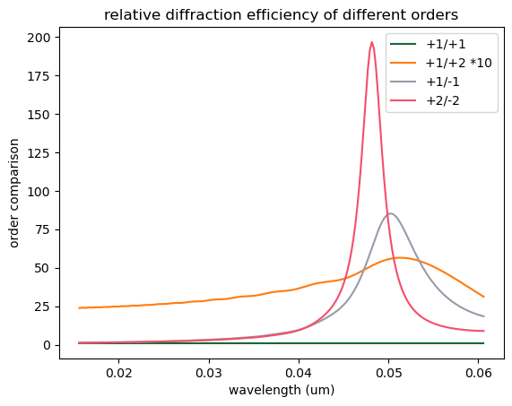
Load the results and compare the efficiency of the different diffraction orders:
#%% load simulation data from file,
# plot and compare the diffraction efficiency of the different orders
sim_data = td.SimulationData.from_file(
    fname='data/diffraction_efficiency.hdf5')  # type:ignore

diffraction_data = sim_data['diffraction_monitor']

E_theta = diffraction_data.Etheta
E_phi = diffraction_data.Ephi

I_proj_theta_0 = (np.abs(E_theta)**2).sel(orders_x=0, orders_y=0)
I_proj_theta_p1 = (np.abs(E_theta)**2).sel(orders_x=1, orders_y=0)
I_proj_theta_p2 = (np.abs(E_theta)**2).sel(orders_x=2, orders_y=0)
I_proj_theta_m1 = (np.abs(E_theta)**2).sel(orders_x=-1, orders_y=0)
I_proj_theta_m2 = (np.abs(E_theta)**2).sel(orders_x=-2, orders_y=0)
I_proj_theta_all = (
    np.abs(E_theta)**2
    ).sum(dim='orders_x', skipna=True
    ).sum(dim='orders_y',skipna=True)

I_theta_proj_0 = I_proj_theta_0/I_proj_theta_all
I_theta_p1 = I_proj_theta_p1/I_proj_theta_all
I_theta_p2 = I_proj_theta_p2/I_proj_theta_all
I_theta_m1 = I_proj_theta_m1/I_proj_theta_all
I_theta_m2 = I_proj_theta_m2/I_proj_theta_all

plt.plot(wls, I_theta_p1, label='+1')
plt.plot(wls, I_theta_p2, label='+2')
plt.plot(wls, I_theta_m1, label='-1')
plt.plot(wls, I_theta_m2, label='-2')
plt.plot(wls, I_theta_proj_0, label='0')
plt.legend()
plt.xlabel('wavelength (um)')
plt.ylabel('diffraction efficiency')
plt.title('absolute diffraction efficiency of different orders')
plt.show()

plt.plot(wls, I_theta_p1/I_theta_p1, label='+1/+1')
plt.plot(wls, I_theta_p1/I_theta_p2*10, label='+1/+2 *10')
plt.plot(wls, I_theta_p1/I_theta_m1, label='+1/-1')
plt.plot(wls, I_theta_p2/I_theta_m2, label='+2/-2')
plt.legend()
plt.xlabel('wavelength (um)')
plt.ylabel('order comparison')
plt.title('relative diffraction efficiency of different orders')
plt.show()


 TERMS & CONDITIONS


 How the process works:
 Try this real URL to see an example: