Authors: Mariia Stepanova, Joshua Bocanegra, Ping-Chun Chen, Melika Momenzadeh, Yingshuo Lyu — Shcherbakov Nanophotonics Lab, University of California, Irvine.
The notebook is focused on designing the following components for the on-chip tunable laser in the visible spectral range:
- GaAs/AlGaAs laser specific to 720-750 nm
- Inverse wedge edge coupler
- Vernier Ring Resonator
- Diffraction Grating Far-field Coupler
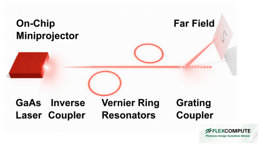
System-level concept for the on-chip tunable laser and passive Vernier filtering architecture.
1. Integrated Laser
Integrated GaAs/AlGaAs Quantum-Well Laser
Active Region Design and 3D FDTD Verification
This notebook models the passive optical cavity / waveguide section of an integrated GaAs/AlGaAs laser using Tidy3D FDTD.
The structure represents a ridge-like III–V laser stack with:
- AlGaAs cladding layers for vertical optical confinement
- AlGaAs waveguide/core layers around the active region
- Three GaAs quantum wells (QWs) modeled as gain layers
- Anti-reflection (AR) coating stacks on the input and output facets
- A fundamental mode source launched along the +x direction
- Flux, mode, and field monitors for transmission and confinement analysis
The main goal is to evaluate how efficiently the guided mode propagates through the active laser section and how strongly the optical field overlaps with the quantum-well gain region near the design wavelength of approximately 731 nm.
The workflow has three stages:
- Define the complete GaAs/AlGaAs epitaxial stack.
- Build a full 3D FDTD model.
- Analyze:
- output-to-input power ratio,
- transmission in dB,
- output modal content,
- optical field confinement.
# ============================================================
# Colab setup
# ============================================================

# Run this only if Tidy3D is not already installed.
# In Google Colab, uncomment:
# !pip install tidy3d

# After installation, configure your FlexCompute API key once:
# import tidy3d.web as web
# web.configure("YOUR_API_KEY")


# ============================================================
# 1. Imports and simulation controls
# ============================================================

from pathlib import Path

import numpy as np
import matplotlib.pyplot as plt
import tidy3d as td
import tidy3d.web as web
from tidy3d.components.grid.mesher import GradedMesher

PROJECT_ROOT = Path.cwd().resolve()
DATA_DIR = PROJECT_ROOT / "data"
DATA_DIR.mkdir(parents=True, exist_ok=True)

SIM_DATA_PATH = DATA_DIR / "sim_data.hdf5"

TASK_NAME = "three_QW_GaAs_AlGaAs_731nm_FDTD"
16:39:19 -03 WARNING: Using canonical configuration directory at
             '/home/filipe/.config/tidy3d'. Found legacy directory at
             '~/.tidy3d', which will be ignored. Remove it manually or run
             'tidy3d config migrate --delete-legacy' to clean up.
1.1 Optical Source and Monitors
The simulation injects a guided mode from the left facet and measures the transmitted optical power at the right facet.
The wavelength range is:
$$ \lambda = 722\text{–}740~\mathrm{nm} $$
which covers the target laser wavelength near:
$$ \lambda_0 \approx 731~\mathrm{nm} $$
The main monitors are:
-
flux_in: input/reference optical power, -
flux_out: transmitted optical power, -
mode_output: output modal decomposition, -
field_xz: longitudinal field profile, -
field_yz_output: output facet field profile.
# ============================================================
# 2. Source and monitor definitions
# ============================================================

air = td.Medium(name="air")

_sort = td.ModeSortSpec(
    filter_reference=0,
    filter_order="over",
    sort_key="n_eff",
    track_freq="central",
    keep_modes="all",
)

# Frequency samples corresponding approximately to 722–740 nm
_freqs = td.C_0 / np.linspace(0.7219753086419753, 0.740253164556962, 15)

fundamental_mode_source = td.ModeSource(
    name="fundamental_mode_source",
    center=[-3.6, 0, 0],
    size=[0, 3, 2.4],
    source_time=td.GaussianPulse(
        freq0=410112801641586.9,
        fwidth=10252820041039.672,
    ),
    direction="+",
    mode_spec=td.ModeSpec(num_modes=3, sort_spec=_sort),
)

field_xz = td.FieldMonitor(
    size=[td.inf, 0, td.inf],
    name="field_xz",
    freqs=_freqs,
    apodization=td.ApodizationSpec(),
)

field_yz_output = td.FieldMonitor(
    center=[3.6, 0, 0],
    size=[0, td.inf, td.inf],
    name="field_yz_output",
    freqs=_freqs,
    apodization=td.ApodizationSpec(),
)

flux_in = td.FluxMonitor(
    center=[-3.6, 0, 0],
    size=[0, 3, 2.4],
    name="flux_in",
    freqs=_freqs,
    apodization=td.ApodizationSpec(),
    normal_dir="+",
)

flux_out = td.FluxMonitor(
    center=[3.6, 0, 0],
    size=[0, 3, 2.4],
    name="flux_out",
    freqs=_freqs,
    apodization=td.ApodizationSpec(),
    normal_dir="+",
)

mode_output = td.ModeMonitor(
    center=[3.6, 0, 0],
    size=[0, 3, 2.4],
    name="mode_output",
    freqs=_freqs,
    apodization=td.ApodizationSpec(),
    mode_spec=td.ModeSpec(num_modes=5, sort_spec=_sort),
    store_fields_direction="+",
)

field_xy = td.FieldMonitor(
    center=[0, 0, 0],
    size=[td.inf, td.inf, 0],
    name="field_xy",
    freqs=_freqs,
    apodization=td.ApodizationSpec(),
)
1.2 Layer Stack and Active Quantum Wells
The laser stack is defined as a sequence of rectangular layers along the vertical z direction.
The active region contains three GaAs quantum wells:
$$ t_\mathrm{QW}=8~\mathrm{nm}=0.008~\mu\mathrm{m} $$
The QWs are surrounded by AlGaAs barriers and waveguide layers. In this model, the QW material is assigned allow_gain=True with a negative conductivity, so it represents optical gain phenomenologically.
This is useful for checking whether the guided optical mode overlaps well with the active region before adding more advanced physics such as carrier transport, thermal effects, or laser rate equations.
# ============================================================
# 3. Material and epitaxial layer definitions
# ============================================================

AlGaAs_cladding = td.Medium(
    name="AlGaAs_cladding",
    permittivity=9.9225,
)

AlGaAs_waveguide_core = td.Medium(
    name="AlGaAs_waveguide_core",
    permittivity=11.902500000000002,
)

GaAs_QW_gain = td.Medium(
    name="GaAs_QW_gain",
    allow_gain=True,
    permittivity=13.322491330706224,
    conductivity=-0.0004903956897612369,
)

GaAs_passive = td.Medium(
    name="GaAs_passive",
    permittivity=13.3225,
)

AR_stack_high_index = td.Medium(
    name="AR_stack_high_index",
    permittivity=6,
)

AR_stack_low_index = td.Medium(
    name="AR_stack_low_index",
    permittivity=2.25,
)

n_doped_AlGaAs_cladding = td.Structure(
    geometry=td.Box(center=[0, 0, -0.512], size=[8, 1, 0.8]),
    name="n_doped_AlGaAs_cladding",
    medium=AlGaAs_cladding,
)

lower_AlGaAs_waveguide_layer = td.Structure(
    geometry=td.Box(center=[0, 0, -0.072], size=[8, 1, 0.08]),
    name="lower_AlGaAs_waveguide_layer",
    medium=AlGaAs_waveguide_core,
)

lower_barrier = td.Structure(
    geometry=td.Box(center=[0, 0, -0.027], size=[8, 1, 0.01]),
    name="lower_barrier",
    medium=AlGaAs_waveguide_core,
)

QW1_gain = td.Structure(
    geometry=td.Box(center=[0, 0, -0.018], size=[8, 1, 0.008]),
    name="QW1_gain",
    medium=GaAs_QW_gain,
)

barrier_QW1_QW2 = td.Structure(
    geometry=td.Box(center=[0, 0, -0.009], size=[8, 1, 0.01]),
    name="barrier_QW1_QW2",
    medium=AlGaAs_waveguide_core,
)

QW2_gain = td.Structure(
    geometry=td.Box(center=[0, 0, 0], size=[8, 1, 0.008]),
    name="QW2_gain",
    medium=GaAs_QW_gain,
)

barrier_QW2_QW3 = td.Structure(
    geometry=td.Box(center=[0, 0, 0.009], size=[8, 1, 0.01]),
    name="barrier_QW2_QW3",
    medium=AlGaAs_waveguide_core,
)

QW3_gain = td.Structure(
    geometry=td.Box(center=[0, 0, 0.018], size=[8, 1, 0.008]),
    name="QW3_gain",
    medium=GaAs_QW_gain,
)

upper_barrier = td.Structure(
    geometry=td.Box(center=[0, 0, 0.027], size=[8, 1, 0.01]),
    name="upper_barrier",
    medium=AlGaAs_waveguide_core,
)

upper_AlGaAs_waveguide_layer = td.Structure(
    geometry=td.Box(center=[0, 0, 0.072], size=[8, 1, 0.08]),
    name="upper_AlGaAs_waveguide_layer",
    medium=AlGaAs_waveguide_core,
)

p_doped_AlGaAs_cladding = td.Structure(
    geometry=td.Box(center=[0, 0, 0.512], size=[8, 1, 0.8]),
    name="p_doped_AlGaAs_cladding",
    medium=AlGaAs_cladding,
)

p_plus_GaAs_contact = td.Structure(
    geometry=td.Box(center=[0, 0, 0.962], size=[8, 1, 0.1]),
    name="p_plus_GaAs_contact",
    medium=GaAs_passive,
)

AR_minus_x_layer1_high = td.Structure(
    geometry=td.Box(center=[-4.0375, 0, 0], size=[0.075, 3, 2.4]),
    name="AR_minus_x_layer1_high",
    medium=AR_stack_high_index,
)

AR_minus_x_layer2_low = td.Structure(
    geometry=td.Box(center=[-4.1365, 0, 0], size=[0.123, 3, 2.4]),
    name="AR_minus_x_layer2_low",
    medium=AR_stack_low_index,
)

AR_plus_x_layer1_high = td.Structure(
    geometry=td.Box(center=[4.0375, 0, 0], size=[0.075, 3, 2.4]),
    name="AR_plus_x_layer1_high",
    medium=AR_stack_high_index,
)

AR_plus_x_layer2_low = td.Structure(
    geometry=td.Box(center=[4.1365, 0, 0], size=[0.123, 3, 2.4]),
    name="AR_plus_x_layer2_low",
    medium=AR_stack_low_index,
)

structures = [
    n_doped_AlGaAs_cladding,
    lower_AlGaAs_waveguide_layer,
    lower_barrier,
    QW1_gain,
    barrier_QW1_QW2,
    QW2_gain,
    barrier_QW2_QW3,
    QW3_gain,
    upper_barrier,
    upper_AlGaAs_waveguide_layer,
    p_doped_AlGaAs_cladding,
    p_plus_GaAs_contact,
    AR_minus_x_layer1_high,
    AR_minus_x_layer2_low,
    AR_plus_x_layer1_high,
    AR_plus_x_layer2_low,
]
layer_summary = [
    ("n-doped AlGaAs cladding", -0.512, 0.800, "AlGaAs cladding"),
    ("lower AlGaAs waveguide", -0.072, 0.080, "AlGaAs core"),
    ("lower barrier", -0.027, 0.010, "AlGaAs core"),
    ("GaAs QW1 gain", -0.018, 0.008, "GaAs gain"),
    ("barrier QW1-QW2", -0.009, 0.010, "AlGaAs core"),
    ("GaAs QW2 gain", 0.000, 0.008, "GaAs gain"),
    ("barrier QW2-QW3", 0.009, 0.010, "AlGaAs core"),
    ("GaAs QW3 gain", 0.018, 0.008, "GaAs gain"),
    ("upper barrier", 0.027, 0.010, "AlGaAs core"),
    ("upper AlGaAs waveguide", 0.072, 0.080, "AlGaAs core"),
    ("p-doped AlGaAs cladding", 0.512, 0.800, "AlGaAs cladding"),
    ("p+ GaAs contact", 0.962, 0.100, "GaAs contact"),
]

print(f"{'Layer':30s} {'z center (µm)':>14s} {'thickness (µm)':>16s}  Material")
print("-" * 86)

for name, zc, thickness, material in layer_summary:
    print(f"{name:30s} {zc:14.3f} {thickness:16.3f}  {material}")
Layer                           z center (µm)   thickness (µm)  Material
--------------------------------------------------------------------------------------
n-doped AlGaAs cladding                -0.512            0.800  AlGaAs cladding
lower AlGaAs waveguide                 -0.072            0.080  AlGaAs core
lower barrier                          -0.027            0.010  AlGaAs core
GaAs QW1 gain                          -0.018            0.008  GaAs gain
barrier QW1-QW2                        -0.009            0.010  AlGaAs core
GaAs QW2 gain                           0.000            0.008  GaAs gain
barrier QW2-QW3                         0.009            0.010  AlGaAs core
GaAs QW3 gain                           0.018            0.008  GaAs gain
upper barrier                           0.027            0.010  AlGaAs core
upper AlGaAs waveguide                  0.072            0.080  AlGaAs core
p-doped AlGaAs cladding                 0.512            0.800  AlGaAs cladding
p+ GaAs contact                         0.962            0.100  GaAs contact
1.3 Mesh Refinement and Full FDTD Simulation
The QWs and barriers are only a few nanometers thick, so vertical mesh refinement is required.
The mesh is refined to:
$$ \Delta z = 2~\mathrm{nm} $$
inside the GaAs quantum wells, and:
$$ \Delta z = 2.5~\mathrm{nm} $$
inside the AlGaAs barriers.
This is important because the confinement factor and gain-overlap calculation are sensitive to the field distribution inside the active region.
# ============================================================
# 4. Mesh overrides and full simulation object
# ============================================================

override_structure_0 = td.MeshOverrideStructure(
    geometry=td.Box(center=[0, 0, -0.018], size=[8, 1, 0.008]),
    name="override_QW1",
    dl=[None, None, 0.002],
)

override_structure_1 = td.MeshOverrideStructure(
    geometry=td.Box(center=[0, 0, 0], size=[8, 1, 0.008]),
    name="override_QW2",
    dl=[None, None, 0.002],
)

override_structure_2 = td.MeshOverrideStructure(
    geometry=td.Box(center=[0, 0, 0.018], size=[8, 1, 0.008]),
    name="override_QW3",
    dl=[None, None, 0.002],
)

override_structure_3 = td.MeshOverrideStructure(
    geometry=td.Box(center=[0, 0, -0.027], size=[8, 1, 0.01]),
    name="override_lower_barrier",
    dl=[None, None, 0.0025],
)

override_structure_4 = td.MeshOverrideStructure(
    geometry=td.Box(center=[0, 0, -0.009], size=[8, 1, 0.01]),
    name="override_barrier_QW1_QW2",
    dl=[None, None, 0.0025],
)

override_structure_5 = td.MeshOverrideStructure(
    geometry=td.Box(center=[0, 0, 0.009], size=[8, 1, 0.01]),
    name="override_barrier_QW2_QW3",
    dl=[None, None, 0.0025],
)

override_structure_6 = td.MeshOverrideStructure(
    geometry=td.Box(center=[0, 0, 0.027], size=[8, 1, 0.01]),
    name="override_upper_barrier",
    dl=[None, None, 0.0025],
)

sim = td.Simulation(
    size=[10, 4, 3],
    boundary_spec=td.BoundarySpec(
        x=td.Boundary(
            plus=td.PML(),
            minus=td.PML(),
        ),
        y=td.Boundary(
            plus=td.PML(),
            minus=td.PML(),
        ),
        z=td.Boundary(
            plus=td.PML(),
            minus=td.PML(),
        ),
    ),
    grid_spec=td.GridSpec(
        grid_x=td.AutoGrid(mesher=GradedMesher(), min_steps_per_wvl=24),
        grid_y=td.AutoGrid(mesher=GradedMesher(), min_steps_per_wvl=24),
        grid_z=td.AutoGrid(mesher=GradedMesher(), min_steps_per_wvl=24),
        wavelength=0.731,
        override_structures=[
            override_structure_0,
            override_structure_1,
            override_structure_2,
            override_structure_3,
            override_structure_4,
            override_structure_5,
            override_structure_6,
        ],
    ),
    run_time=3e-12,
    medium=air,
    sources=[fundamental_mode_source],
    monitors=[field_xz, field_yz_output, flux_in, flux_out, mode_output, field_xy],
    structures=structures,
)

sim
16:39:21 -03 WARNING: Structure: 'AR_minus_x_layer1_high'
             (simulation.structures[12]) was detected as being less than half of
             a central wavelength from a PML on side z-min. To avoid inaccurate
             results or divergence, please increase gap between any structures
             and PML or fully extend structure through the pml.
WARNING: Suppressed 7 WARNING messages.
Simulation(center=(0.0, 0.0, 0.0), size=(10.0, 4.0, 3.0), medium=air, structures=(Structure(geometry=Box(center=(0.0, 0.0, -0.512), size=(8.0, 1.0, 0.8)), name='n_doped_AlGaAs_cladding', background_permittivity=None, background_medium=None, priority=None,medium=AlGaAs_cladding), Structure(geometry=Box(center=(0.0, 0.0, -0.072), size=(8.0, 1.0, 0.08)), name='lower_AlGaAs_waveguide_layer', background_permittivity=None, background_medium=None, priority=None,medium=AlGaAs_waveguide_core), Structure(geometry=Box(center=(0.0, 0.0, -0.027), size=(8.0, 1.0, 0.01)), name='lower_barrier', background_permittivity=None, background_medium=None, priority=None,medium=AlGaAs_waveguide_core), Structure(geometry=Box(center=(0.0, 0.0, -0.018), size=(8.0, 1.0, 0.008)), name='QW1_gain', background_permittivity=None, background_medium=None, priority=None,medium=GaAs_QW_gain), Structure(geometry=Box(center=(0.0, 0.0, -0.009), size=(8.0, 1.0, 0.01)), name='barrier_QW1_QW2', background_permittivity=None, background_medium=None, priority=None,medium=AlGaAs_waveguide_core), Structure(geometry=Box(center=(0.0, 0.0, 0.0), size=(8.0, 1.0, 0.008)), name='QW2_gain', background_permittivity=None, background_medium=None, priority=None,medium=GaAs_QW_gain), Structure(geometry=Box(center=(0.0, 0.0, 0.009), size=(8.0, 1.0, 0.01)), name='barrier_QW2_QW3', background_permittivity=None, background_medium=None, priority=None,medium=AlGaAs_waveguide_core), Structure(geometry=Box(center=(0.0, 0.0, 0.018), size=(8.0, 1.0, 0.008)), name='QW3_gain', background_permittivity=None, background_medium=None, priority=None,medium=GaAs_QW_gain), Structure(geometry=Box(center=(0.0, 0.0, 0.027), size=(8.0, 1.0, 0.01)), name='upper_barrier', background_permittivity=None, background_medium=None, priority=None,medium=AlGaAs_waveguide_core), Structure(geometry=Box(center=(0.0, 0.0, 0.072), size=(8.0, 1.0, 0.08)), name='upper_AlGaAs_waveguide_layer', background_permittivity=None, background_medium=None, priority=None,medium=AlGaAs_waveguide_core), Structure(geometry=Box(center=(0.0, 0.0, 0.512), size=(8.0, 1.0, 0.8)), name='p_doped_AlGaAs_cladding', background_permittivity=None, background_medium=None, priority=None,medium=AlGaAs_cladding), Structure(geometry=Box(center=(0.0, 0.0, 0.962), size=(8.0, 1.0, 0.1)), name='p_plus_GaAs_contact', background_permittivity=None, background_medium=None, priority=None,medium=GaAs_passive), Structure(geometry=Box(center=(-4.0375, 0.0, 0.0), size=(0.075, 3.0, 2.4)), name='AR_minus_x_layer1_high', background_permittivity=None, background_medium=None, priority=None,medium=AR_stack_high_index), Structure(geometry=Box(center=(-4.1365, 0.0, 0.0), size=(0.123, 3.0, 2.4)), name='AR_minus_x_layer2_low', background_permittivity=None, background_medium=None, priority=None,medium=AR_stack_low_index), Structure(geometry=Box(center=(4.0375, 0.0, 0.0), size=(0.075, 3.0, 2.4)), name='AR_plus_x_layer1_high', background_permittivity=None, background_medium=None, priority=None,medium=AR_stack_high_index), Structure(geometry=Box(center=(4.1365, 0.0, 0.0), size=(0.123, 3.0, 2.4)), name='AR_plus_x_layer2_low', background_permittivity=None, background_medium=None, priority=None,medium=AR_stack_low_index)), symmetry=(0, 0, 0), sources=(ModeSource(name='fundamental_mode_source',center=(-3.6, 0.0, 0.0), size=(0.0, 3.0, 2.4), source_time=GaussianPulse(amplitude=1.0, phase=0.0,freq0=410112801641586.9, fwidth=10252820041039.672, offset=5.0, remove_dc_component=True), num_freqs=1, broadband_method='chebyshev', use_colocated_integration=True, direction='+', mode_spec=ModeSpec(num_modes=3), frame=None, mode_index=0)), boundary_spec=BoundarySpec(), monitors=(FieldMonitor(center=(0.0, 0.0, 0.0), size=(inf, 0.0, inf), name='field_xz', interval_space=(1, 1, 1), colocate=True, use_colocated_integration=True, freqs=array([4.15239212e+14, 4.14489682e+14, 4.13742854e+14, 4.12998712e+14, 4.12257242e+14, 4.11518430e+14, 4.10782261e+14, 4.10048722e+14, 4.09317797e+14, 4.08589473e+14, 4.07863737e+14, 4.07140575e+14, 4.06419972e+14, 4.05701915e+14, 4.04986392e+14]), apodization=ApodizationSpec(), fields=('Ex', 'Ey', 'Ez', 'Hx', 'Hy', 'Hz')), FieldMonitor(center=(3.6, 0.0, 0.0), size=(0.0, inf, inf), name='field_yz_output', interval_space=(1, 1, 1), colocate=True, use_colocated_integration=True, freqs=array([4.15239212e+14, 4.14489682e+14, 4.13742854e+14, 4.12998712e+14, 4.12257242e+14, 4.11518430e+14, 4.10782261e+14, 4.10048722e+14, 4.09317797e+14, 4.08589473e+14, 4.07863737e+14, 4.07140575e+14, 4.06419972e+14, 4.05701915e+14, 4.04986392e+14]), apodization=ApodizationSpec(), fields=('Ex', 'Ey', 'Ez', 'Hx', 'Hy', 'Hz')), FluxMonitor(center=(-3.6, 0.0, 0.0), size=(0.0, 3.0, 2.4), name='flux_in', interval_space=(1, 1, 1), colocate=True, use_colocated_integration=True, freqs=array([4.15239212e+14, 4.14489682e+14, 4.13742854e+14, 4.12998712e+14, 4.12257242e+14, 4.11518430e+14, 4.10782261e+14, 4.10048722e+14, 4.09317797e+14, 4.08589473e+14, 4.07863737e+14, 4.07140575e+14, 4.06419972e+14, 4.05701915e+14, 4.04986392e+14]), apodization=ApodizationSpec(), normal_dir='+', exclude_surfaces=None), FluxMonitor(center=(3.6, 0.0, 0.0), size=(0.0, 3.0, 2.4), name='flux_out', interval_space=(1, 1, 1), colocate=True, use_colocated_integration=True, freqs=array([4.15239212e+14, 4.14489682e+14, 4.13742854e+14, 4.12998712e+14, 4.12257242e+14, 4.11518430e+14, 4.10782261e+14, 4.10048722e+14, 4.09317797e+14, 4.08589473e+14, 4.07863737e+14, 4.07140575e+14, 4.06419972e+14, 4.05701915e+14, 4.04986392e+14]), apodization=ApodizationSpec(), normal_dir='+', exclude_surfaces=None), ModeMonitor(center=(3.6, 0.0, 0.0), size=(0.0, 3.0, 2.4), name='mode_output', interval_space=(1, 1, 1), colocate=True, use_colocated_integration=True, freqs=array([4.15239212e+14, 4.14489682e+14, 4.13742854e+14, 4.12998712e+14, 4.12257242e+14, 4.11518430e+14, 4.10782261e+14, 4.10048722e+14, 4.09317797e+14, 4.08589473e+14, 4.07863737e+14, 4.07140575e+14, 4.06419972e+14, 4.05701915e+14, 4.04986392e+14]), apodization=ApodizationSpec(), store_fields_direction='+', conjugated_dot_product=True, mode_spec=ModeSpec(num_modes=5)), FieldMonitor(center=(0.0, 0.0, 0.0), size=(inf, inf, 0.0), name='field_xy', interval_space=(1, 1, 1), colocate=True, use_colocated_integration=True, freqs=array([4.15239212e+14, 4.14489682e+14, 4.13742854e+14, 4.12998712e+14, 4.12257242e+14, 4.11518430e+14, 4.10782261e+14, 4.10048722e+14, 4.09317797e+14, 4.08589473e+14, 4.07863737e+14, 4.07140575e+14, 4.06419972e+14, 4.05701915e+14, 4.04986392e+14]), apodization=ApodizationSpec(), fields=('Ex', 'Ey', 'Ez', 'Hx', 'Hy', 'Hz'))), grid_spec=GridSpec(grid_x=AutoGrid(min_steps_per_wvl=24.0), grid_y=AutoGrid(min_steps_per_wvl=24.0), grid_z=AutoGrid(min_steps_per_wvl=24.0), wavelength=0.731, override_structures=(MeshOverrideStructure(geometry=Box(center=(0.0, 0.0, -0.018), size=(8.0, 1.0, 0.008)), name='override_QW1', background_permittivity=None, background_medium=None, priority=0,dl=(None, None, 0.002), enforce=False, shadow=True, drop_outside_sim=True), MeshOverrideStructure(geometry=Box(center=(0.0, 0.0, 0.0), size=(8.0, 1.0, 0.008)), name='override_QW2', background_permittivity=None, background_medium=None, priority=0,dl=(None, None, 0.002), enforce=False, shadow=True, drop_outside_sim=True), MeshOverrideStructure(geometry=Box(center=(0.0, 0.0, 0.018), size=(8.0, 1.0, 0.008)), name='override_QW3', background_permittivity=None, background_medium=None, priority=0,dl=(None, None, 0.002), enforce=False, shadow=True, drop_outside_sim=True), MeshOverrideStructure(geometry=Box(center=(0.0, 0.0, -0.027), size=(8.0, 1.0, 0.01)), name='override_lower_barrier', background_permittivity=None, background_medium=None, priority=0,dl=(None, None, 0.0025), enforce=False, shadow=True, drop_outside_sim=True), MeshOverrideStructure(geometry=Box(center=(0.0, 0.0, -0.009), size=(8.0, 1.0, 0.01)), name='override_barrier_QW1_QW2', background_permittivity=None, background_medium=None, priority=0,dl=(None, None, 0.0025), enforce=False, shadow=True, drop_outside_sim=True), MeshOverrideStructure(geometry=Box(center=(0.0, 0.0, 0.009), size=(8.0, 1.0, 0.01)), name='override_barrier_QW2_QW3', background_permittivity=None, background_medium=None, priority=0,dl=(None, None, 0.0025), enforce=False, shadow=True, drop_outside_sim=True), MeshOverrideStructure(geometry=Box(center=(0.0, 0.0, 0.027), size=(8.0, 1.0, 0.01)), name='override_upper_barrier', background_permittivity=None, background_medium=None, priority=0,dl=(None, None, 0.0025), enforce=False, shadow=True, drop_outside_sim=True))), version='2.11.2', plot_length_units='μm', structure_priority_mode='equal', lumped_elements=(), subpixel=SubpixelSpec(), simulation_type='tidy3d', post_norm=1.0, internal_absorbers=(), courant=0.99, relax_courant=False, precision='hybrid', normalize_index=0, shutoff=1e-05, run_time=3e-12, low_freq_smoothing=None)
# Sanity checks before launching the solver

print("Simulation domain size (µm):", sim.size)
print("Run time (s):", sim.run_time)
print("Number of structures:", len(sim.structures))
print("Number of monitors:", len(sim.monitors))
print("Number of sources:", len(sim.sources))

try:
    print(sim.grid_info)
except Exception as exc:
    print("Grid info is not available in this Tidy3D version.")
    print("Reason:", exc)
Simulation domain size (µm): (10.0, 4.0, 3.0)
Run time (s): 3e-12
Number of structures: 16
Number of monitors: 6
Number of sources: 1
{'Nx': 1065, 'Ny': 342, 'Nz': 322, 'grid_points': 117282060, 'min_grid_size': 0.0017391304347826875, 'max_grid_size': 0.030458333333333698, 'computational_complexity': 67437184499.99695, 'fine_mesh_info': ['z=-0.02461 (size=0.001739)', 'z=-0.02287 (size=0.001739)', 'z=-0.01309 (size=0.001818)', 'z=-0.01127 (size=0.001818)', 'z=-0.004909 (size=0.001818)', 'z=0.004909 (size=0.001818)', 'z=0.006727 (size=0.001818)', 'z=0.01309 (size=0.001818)', 'z=0.02287 (size=0.001739)', 'z=0.02461 (size=0.001739)']}
# Geometry cross-sections of the laser stack.
fig, axes = plt.subplots(1, 2, figsize=(12, 4))
sim.plot(y=0, ax=axes[0])
axes[0].set_title("Vertical x-z cross-section: 3-QW GaAs/AlGaAs laser")
sim.plot(x=0, ax=axes[1])
axes[1].set_title("Transverse y-z cross-section")
plt.tight_layout()
plt.show()

sim.plot_3d()
1.4 Run or Load Simulation Data
If data/sim_data.hdf5 already exists, the notebook loads the saved result from disk. Otherwise, it submits a new simulation to FlexCompute and saves the result there for later post-processing.
# ============================================================
# 5. Run or load simulation data
# ============================================================

if SIM_DATA_PATH.exists():
    sim_data = td.SimulationData.from_file(str(SIM_DATA_PATH))
    print("Loaded simulation data from:", SIM_DATA_PATH)
else:
    sim_data = web.run(
        sim,
        task_name=TASK_NAME,
        path=str(SIM_DATA_PATH),
        verbose=True,
    )
    print("Saved simulation data to:", SIM_DATA_PATH)

if getattr(sim_data, "diverged", False):
    print("Warning: simulation diverged.")
16:39:26 -03 WARNING: Structure: 'AR_minus_x_layer1_high'
             (simulation.structures[12]) was detected as being less than half of
             a central wavelength from a PML on side z-min. To avoid inaccurate
             results or divergence, please increase gap between any structures
             and PML or fully extend structure through the pml.
WARNING: Suppressed 7 WARNING messages.
Loaded simulation data from: /home/filipe/Desktop/GITHUB/tidyvernier-dual-ring-filter/tidy3d-community-library/notebooks/data/sim_data.hdf5
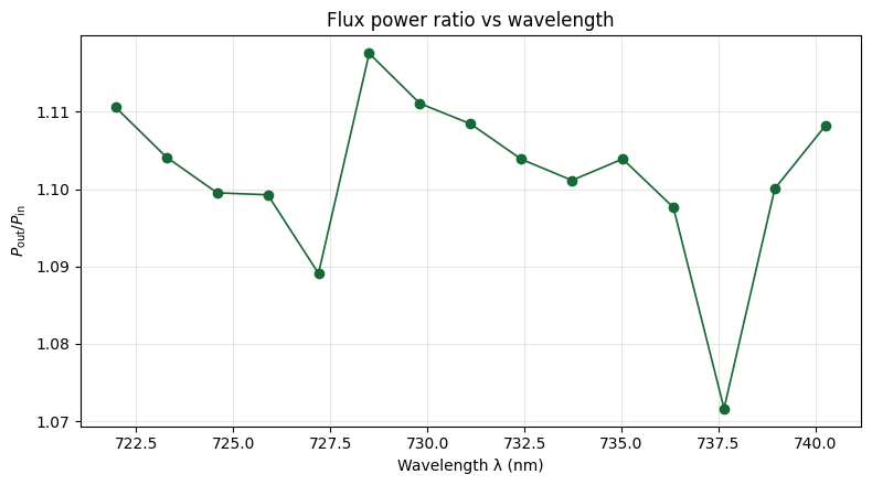
1.5 Output-to-Input Power Ratio
The wavelength-dependent transmission is calculated as:
$$ T(\lambda)=\frac{P_\mathrm{out}(\lambda)}{P_\mathrm{in}(\lambda)} $$
where P_in and P_out are measured by the input and output flux monitors.
For a passive waveguide, $T<1$ indicates propagation loss, scattering loss, facet loss, or mode mismatch.
With gain enabled, $T>1$ can indicate that the modal gain is larger than the total loss.
# ============================================================
# 6. Transmission spectrum
# ============================================================

fin = sim_data["flux_in"].flux
fout = sim_data["flux_out"].flux

f_hz = np.asarray(fin.f.values, dtype=float).ravel()
wavelength_um = float(td.C_0) / f_hz

pin = np.abs(np.asarray(fin.values, dtype=np.complex128).ravel())
pout = np.abs(np.asarray(fout.values, dtype=np.complex128).ravel())

T = np.where(pin > 0, pout / pin, np.nan)

order = np.argsort(wavelength_um)
wl_um = wavelength_um[order]
T = T[order]

fig, ax = plt.subplots(figsize=(8, 4.5))
ax.plot(wl_um * 1e3, T, "o-", lw=1.2, ms=6)
ax.set_xlabel("Wavelength λ (nm)")
ax.set_ylabel(r"$P_\mathrm{out}/P_\mathrm{in}$")
ax.set_title("Flux power ratio vs wavelength")
ax.grid(True, alpha=0.3)
plt.tight_layout()
plt.show()
# Transmission in dB

T_dB = 10 * np.log10(np.maximum(T, 1e-30))

fig, ax = plt.subplots(figsize=(8, 4.5))
ax.plot(wl_um * 1e3, T_dB, "o-", lw=1.2, ms=6)
ax.set_xlabel("Wavelength λ (nm)")
ax.set_ylabel(r"$10\log_{10}(P_\mathrm{out}/P_\mathrm{in})$ (dB)")
ax.set_title("Integrated GaAs/AlGaAs laser section: net power transfer")
ax.grid(True, alpha=0.3)
plt.tight_layout()
plt.show()

best_idx = np.nanargmax(T)
print(f"Peak transfer = {T[best_idx]:.3g}")
print(f"Peak transfer = {T_dB[best_idx]:.2f} dB")
print(f"Peak wavelength = {wl_um[best_idx] * 1e3:.2f} nm")
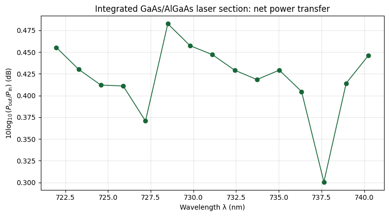
Peak transfer = 1.12
Peak transfer = 0.48 dB
Peak wavelength = 728.50 nm
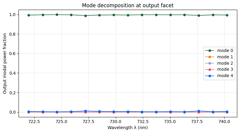
1.6 Modal Content at the Output
The mode_output monitor decomposes the transmitted field into guided modes.
The modal fraction of mode $m$ is:
$$ \eta_m(\lambda)= \frac{|a_m(\lambda)|^2}{\sum_m |a_m(\lambda)|^2} $$
This confirms whether the output power remains mostly in the desired fundamental guided mode or is scattered into higher-order modes.
# ============================================================
# 7. Output mode decomposition
# ============================================================

try:
    mode_data = sim_data["mode_output"]
    amps = mode_data.amps

    if "direction" in amps.dims or "direction" in amps.coords:
        try:
            amps = amps.sel(direction="+")
        except Exception:
            pass

    amp_values = np.asarray(amps.values)
    dims = list(amps.dims)

    f_axis = dims.index("f") if "f" in dims else 0
    mode_axis = dims.index("mode_index") if "mode_index" in dims else -1

    amp_values = np.moveaxis(amp_values, f_axis, 0)

    dims_moved = [dims[f_axis]] + [d for j, d in enumerate(dims) if j != f_axis]

    if "mode_index" in dims_moved:
        mode_axis_new = dims_moved.index("mode_index")
        amp_values = np.moveaxis(amp_values, mode_axis_new, 1)

    modal_power = np.abs(amp_values) ** 2

    if modal_power.ndim > 2:
        modal_power = modal_power.reshape(
            modal_power.shape[0],
            modal_power.shape[1],
            -1,
        ).sum(axis=-1)

    f_mode = np.asarray(amps.f.values, dtype=float).ravel()
    wl_mode_nm = float(td.C_0) / f_mode * 1e3

    order_m = np.argsort(wl_mode_nm)
    wl_mode_nm = wl_mode_nm[order_m]
    modal_power = modal_power[order_m, :]

    modal_fraction = modal_power / np.maximum(
        modal_power.sum(axis=1, keepdims=True),
        1e-30,
    )

    fig, ax = plt.subplots(figsize=(8, 4.5))

    max_modes_to_plot = min(5, modal_fraction.shape[1])

    for m in range(max_modes_to_plot):
        ax.plot(
            wl_mode_nm,
            modal_fraction[:, m],
            "o-",
            lw=1.2,
            ms=5,
            label=f"mode {m}",
        )

    ax.set_xlabel("Wavelength λ (nm)")
    ax.set_ylabel("Output modal power fraction")
    ax.set_title("Mode decomposition at output facet")
    ax.grid(True, alpha=0.3)
    ax.legend()
    plt.tight_layout()
    plt.show()

except Exception as exc:
    print("Could not extract modal decomposition from mode_output.")
    print("Reason:", exc)
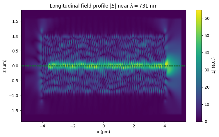
1.7 Field Visualization
The electric-field magnitude is calculated as:
$$ |E|=\sqrt{|E_x|^2+|E_y|^2+|E_z|^2} $$
The longitudinal x-z field map is useful for checking:
- confinement inside the waveguide core,
- overlap with the GaAs quantum wells,
- leakage into the cladding,
- standing-wave or reflection behavior.
# ============================================================
# 8. Field visualization near 731 nm
# ============================================================

design_wavelength_um = 0.731

try:
    field = sim_data["field_xz"]
    f_target = float(td.C_0) / design_wavelength_um

    Ex = field.Ex.sel(f=f_target, method="nearest")
    Ey = field.Ey.sel(f=f_target, method="nearest")
    Ez = field.Ez.sel(f=f_target, method="nearest")

    E_mag = np.sqrt(
        np.abs(Ex.values) ** 2 + np.abs(Ey.values) ** 2 + np.abs(Ez.values) ** 2
    )

    E_plot = np.squeeze(E_mag)

    x = np.asarray(Ex.x.values, dtype=float)
    z = np.asarray(Ex.z.values, dtype=float)

    fig, ax = plt.subplots(figsize=(8, 4.8))
    im = ax.pcolormesh(x, z, E_plot.T, shading="auto")

    ax.set_xlabel("x (µm)")
    ax.set_ylabel("z (µm)")
    ax.set_title(r"Longitudinal field profile $|E|$ near $\lambda=731$ nm")

    fig.colorbar(im, ax=ax, label=r"$|E|$ (a.u.)")

    # Mark approximate QW region
    for z_qw in [-0.018, 0.000, 0.018]:
        ax.axhline(z_qw, linestyle="--", linewidth=0.8)

    plt.tight_layout()
    plt.show()

except Exception as exc:
    print("Could not plot field_xz monitor.")
    print("Reason:", exc)
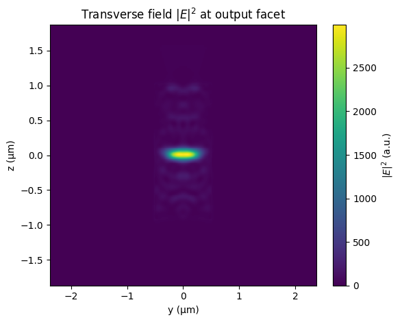
# Transverse field |E|^2 at the output facet near 731 nm.
fyz = sim_data["field_yz_output"]
f_target = float(td.C_0) / design_wavelength_um
Ey0 = fyz.Ey.sel(f=f_target, method="nearest")
E2 = (
    np.abs(fyz.Ex.sel(f=f_target, method="nearest").values) ** 2
    + np.abs(fyz.Ey.sel(f=f_target, method="nearest").values) ** 2
    + np.abs(fyz.Ez.sel(f=f_target, method="nearest").values) ** 2
)
E2 = np.squeeze(E2)
y = np.asarray(Ey0.y.values, dtype=float)
z = np.asarray(Ey0.z.values, dtype=float)
fig, ax = plt.subplots(figsize=(6, 4.8))
im = ax.pcolormesh(y, z, E2.T, shading="auto")
ax.set_xlabel("y (µm)")
ax.set_ylabel("z (µm)")
ax.set_title(r"Transverse field $|E|^2$ at output facet")
fig.colorbar(im, ax=ax, label=r"$|E|^2$ (a.u.)")
plt.tight_layout()
plt.show()
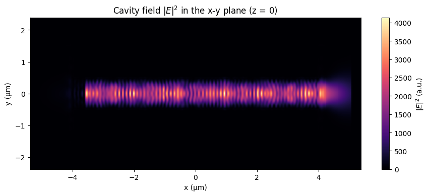
# Cavity standing-wave field |E|^2 in the x-y plane (QW plane, z = 0).
fxy = sim_data["field_xy"]
f_target = float(td.C_0) / design_wavelength_um
E2 = (
    np.abs(fxy.Ex.sel(f=f_target, method="nearest").values) ** 2
    + np.abs(fxy.Ey.sel(f=f_target, method="nearest").values) ** 2
    + np.abs(fxy.Ez.sel(f=f_target, method="nearest").values) ** 2
)
E2 = np.squeeze(E2)
x = np.asarray(fxy.Ex.x.values, dtype=float)
y = np.asarray(fxy.Ex.y.values, dtype=float)
fig, ax = plt.subplots(figsize=(9, 4))
im = ax.pcolormesh(x, y, E2.T, shading="auto", cmap="magma")
ax.set_xlabel("x (µm)")
ax.set_ylabel("y (µm)")
ax.set_title(r"Cavity field $|E|^2$ in the x-y plane (z = 0)")
fig.colorbar(im, ax=ax, label=r"$|E|^2$ (a.u.)")
plt.tight_layout()
plt.show()
1.8 Save the Output Mode Monitor Data
The output mode-monitor amplitudes are written to a compact HDF5 file with Tidy3D's native serializer. A forward modal power/fraction summary is attached through the object's attrs dictionary.
# Save the output mode-monitor data (amplitudes + forward modal summary) to a compact HDF5 file.
# The stored mode fields are dropped here (they remain in sim_data.hdf5), and the extra
# power/fraction calculation is attached via the native `attrs` dictionary.
OUTPUT_MODE_HDF5_PATH = DATA_DIR / "mode_output.hdf5"

mode_data = sim_data["mode_output"]
amps_fwd = mode_data.amps.sel(direction="+")
modal_power = np.moveaxis(
    np.abs(np.asarray(amps_fwd.values)) ** 2, list(amps_fwd.dims).index("f"), 0
)
modal_fraction = modal_power / np.maximum(modal_power.sum(axis=1, keepdims=True), 1e-30)
f_hz = np.asarray(amps_fwd.f.values, dtype=float)

forward_modal_summary = {
    "frequency_hz": f_hz.tolist(),
    "wavelength_um": (td.C_0 / f_hz).tolist(),
    "modal_power": modal_power.tolist(),
    "modal_fraction": modal_fraction.tolist(),
}

stored_fields = {component: None for component in ("Ex", "Ey", "Ez", "Hx", "Hy", "Hz")}
mode_data.updated_copy(
    attrs={"forward_modal_summary": forward_modal_summary}, **stored_fields
).to_hdf5(str(OUTPUT_MODE_HDF5_PATH))
1.9 Conclusion
This simulation provides a compact 3D FDTD model of an integrated GaAs/AlGaAs quantum-well laser section operating near 731 nm.
The active region is represented by three thin GaAs quantum wells embedded between AlGaAs barriers and cladding layers. A guided fundamental mode is launched from the input facet, while flux, mode, and field monitors are used to evaluate the optical response at the output.
The key outputs are:
-
Power transfer spectrum
$$ P_\mathrm{out}/P_\mathrm{in} $$
showing wavelength-dependent gain or loss. -
Transmission in dB
useful for comparing propagation loss, facet loss, and net modal gain. -
Output modal decomposition
confirming whether the transmitted field remains in the desired guided mode. -
Electric-field profiles
verifying confinement and overlap with the quantum-well active region.
Overall, this simulation serves as the integrated-laser building block before coupling the laser output into the rest of the photonic circuit.
2. SiN Waveguide
2.1 Waveguide Design
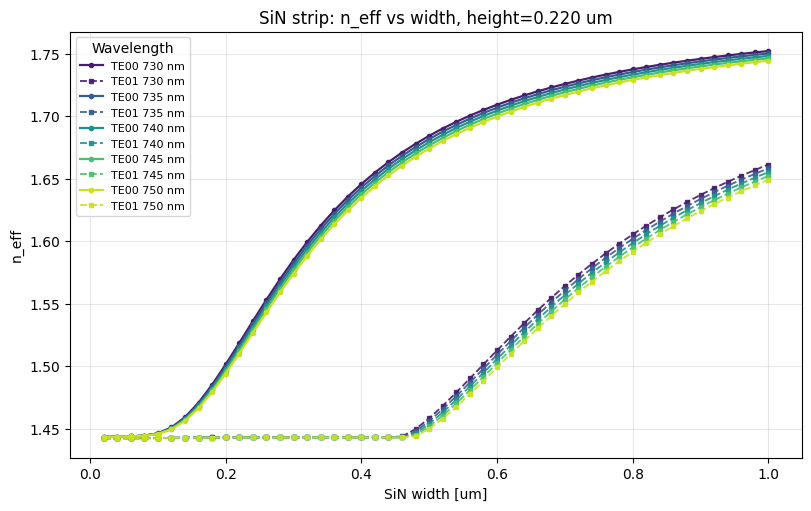
This section sweeps a rectangular SiN strip waveguide embedded in SiO2 and plots the TE00 / TE01 effective-index branches versus waveguide width. Members of our group have familiarity with AIM photonics foundry PDK and wanted to stick within their constraints in order to design a device that could be feasibly manufactured. Thus, we were limited to 220 nm thick SiN.
We omit a schematic here, but the general shape is a rectangle of SiN surrounded by SiO2 cladding. We also assume that the SiN is far enough away from the substrate that we need not include a Si substrate in the simulation results.
import h5py
import xarray as xr
import tidy3d.web.api.mode as mode_web
from tidy3d.plugins.mode import ModeSolver

SIN_SWEEP_DIR = DATA_DIR / "sin_waveguide_sweep_h0220_te_modes"
SIN_SWEEP_HDF5 = SIN_SWEEP_DIR / "passive_sin_mode_sweep.hdf5"
SIN_SWEEP_PNG = SIN_SWEEP_DIR / "plots" / "neff_vs_width_te00_te01.png"
We need to import a few more python libraries in order to continue. HDF5 (h5py) is a common compressed data format that members of the team have used in the past that allows for better storage and read time when compared to csv.
We first build some helper functions in order to create our simulations.
def sin_range(start, stop, step):
    values = []
    current = float(start)
    while current <= float(stop) + 0.5 * float(step):
        values.append(round(current, 6))
        current += float(step)
    return tuple(values)
Generating Data
Simulation space, wavelengths of interest, number of modes, and resolution are all given as parameters. An option to run with or without substrate is given. td.ModeSpec() is a standard function from tidy3d.
def sin_strip_mode_solver(
    width_um,
    *,
    height_um=0.220,
    wavelengths_um=(0.730, 0.735, 0.740, 0.745, 0.750),
    n_sin=2.0,
    n_sio2=1.444,
    n_si=3.8,
    include_si_substrate=False,
    waveguide_bottom_above_si_um=5.0,
    oxide_top_above_si_um=10.0,
    y_span_um=6.0,
    x_span_um=1.0,
    min_steps_per_wvl=20,
    num_modes=3,
    target_neff=1.7,
):
    sin = td.Medium(permittivity=n_sin**2, name="SiN")
    sio2 = td.Medium(permittivity=n_sio2**2, name="SiO2")
    si = td.Medium(permittivity=n_si**2, name="Si")

    core_bottom_z = waveguide_bottom_above_si_um
    core_center_z = core_bottom_z + 0.5 * height_um
    z_min = -1.0
    z_max = oxide_top_above_si_um
    z_center = 0.5 * (z_min + z_max)
    z_span = z_max - z_min

    core_box = td.Box(center=(0, 0, core_center_z), size=(td.inf, width_um, height_um))
    substrate_box = td.Box(center=(0, 0, -0.5), size=(td.inf, td.inf, 1.0))
    structures = [td.Structure(geometry=core_box, medium=sin, name="sin_strip")]
    if include_si_substrate:
        structures.insert(
            0, td.Structure(geometry=substrate_box, medium=si, name="si_substrate")
        )

    sim = td.Simulation(
        center=(0, 0, z_center),
        size=(x_span_um, y_span_um, z_span),
        medium=sio2,
        structures=structures,
        sources=[],
        monitors=[],
        grid_spec=td.GridSpec.auto(
            wavelength=min(wavelengths_um),
            min_steps_per_wvl=min_steps_per_wvl,
        ),
        boundary_spec=td.BoundarySpec(
            x=td.Boundary.periodic(),
            y=td.Boundary.pml(),
            z=td.Boundary.pml(),
        ),
        run_time=1e-12,
    )
    mode_spec = td.ModeSpec(
        num_modes=num_modes,
        target_neff=target_neff,
        sort_spec=td.ModeSortSpec(
            filter_key="TE_fraction",
            filter_reference=0.5,
            filter_order="over",
            sort_key="n_eff",
            sort_order="descending",
            track_freq="central",
        ),
    )
    plane = td.Box(center=(0, 0, z_center), size=(0, y_span_um, z_span))
    solver = ModeSolver(
        simulation=sim,
        plane=plane,
        mode_spec=mode_spec,
        freqs=td.C_0 / np.asarray(wavelengths_um),
        direction="+",
        fields=("Ex", "Ey", "Ez"),
    )
    return solver, core_box, substrate_box
One of the metrics to determine how well the mode is confined inside the waveguide. It is not used in plotting below, but helpful for characterizing sweeps.
def box_intensity_fraction(mode_data, box):
    intensity = mode_data.intensity
    area = mode_data._diff_area
    lower, upper = box.bounds
    mask = None
    for dim in area.dims:
        axis = "xyz".index(dim)
        coords = np.asarray(intensity.coords[dim].values)
        dim_mask = (coords >= lower[axis]) & (coords <= upper[axis])
        mask = dim_mask if mask is None else np.logical_and.outer(mask, dim_mask)
    mask_da = xr.DataArray(
        mask.astype(float),
        coords={dim: intensity.coords[dim].values for dim in area.dims},
        dims=area.dims,
    )
    weighted = intensity * area
    total = weighted.sum(dim=area.dims)
    inside = (weighted * mask_da).sum(dim=area.dims)
    return np.asarray((inside / total.where(total != 0)).fillna(0.0).values)
Main function that runs the sweep for determining the effective index of the mode for the various wavelengths, and sizes of the waveguide. An option to only estimate costs prior to running is included. run_cloud and estimate_cost both default to false in order to prevent accidental use of cloud credits. Ensure that you run the function with estimate_cost set to True to get a cost estimate.
Function can be explicitly run below.
All data is saved as an hdf5 file here. We plot the results after we have the data and it is run as an entirely separate function utilizing matplotlib.
def run_sin_waveguide_sweep(
    *,
    output_dir=SIN_SWEEP_DIR,
    widths_um=sin_range(0.02, 1.00, 0.02),
    height_um=0.220,
    wavelengths_um=(0.730, 0.735, 0.740, 0.745, 0.750),
    run_cloud=False,
    estimate_cost=False,
    cloud_max_workers=20,
    cloud_folder_name="Passive SiN Mode Sweep",
):
    output_dir = Path(output_dir)
    output_dir.mkdir(parents=True, exist_ok=True)
    mode_dir = output_dir / "passive_sin_mode_data"
    mode_dir.mkdir(parents=True, exist_ok=True)
    heights_um = (float(height_um),)
    widths_um = tuple(float(w) for w in widths_um)
    wavelengths_um = tuple(float(w) for w in wavelengths_um)
    shape = (len(widths_um), 1, len(wavelengths_um), 3)

    solvers, records = [], []
    for width_index, width_um in enumerate(widths_um):
        label = f"w{int(round(1000 * width_um)):04d}nm_h{int(round(1000 * height_um)):04d}nm"
        solver, core_box, substrate_box = sin_strip_mode_solver(
            width_um,
            height_um=height_um,
            wavelengths_um=wavelengths_um,
        )
        mode_path = mode_dir / f"{label}.hdf5"
        solvers.append(solver)
        records.append((width_index, core_box, substrate_box, mode_path))

    if estimate_cost:
        costs = np.full((len(widths_um), 1), np.nan)
        task_ids = np.full((len(widths_um), 1), "", dtype=object)
        solver_ids = np.full((len(widths_um), 1), "", dtype=object)
        for solver, (width_index, _, _, _) in zip(solvers, records):
            task = mode_web.ModeSolverTask.create(
                solver,
                task_name=f"estimate_passive_sin_mode_w{int(round(1000 * widths_um[width_index])):04d}",
                mode_solver_name=f"w{int(round(1000 * widths_um[width_index])):04d}",
                folder_name=cloud_folder_name,
            )
            task.upload(verbose=True)
            costs[width_index, 0] = web.estimate_cost(task.task_id, verbose=True)
            task_ids[width_index, 0] = task.task_id or ""
            solver_ids[width_index, 0] = task.solver_id or ""
        cost_path = output_dir / "passive_sin_mode_sweep_cost_estimates.hdf5"
        with h5py.File(cost_path, "w") as h5:
            h5.attrs["total_estimated_flexcredits"] = float(np.nansum(costs))
            h5.create_dataset("wavelength_um", data=np.asarray(wavelengths_um))
            h5.create_dataset("width_um", data=np.asarray(widths_um))
            h5.create_dataset("height_um", data=np.asarray(heights_um))
            h5.create_dataset("estimated_flexcredits", data=costs)
            h5.create_dataset(
                "task_id", data=task_ids, dtype=h5py.string_dtype("utf-8")
            )
            h5.create_dataset(
                "solver_id", data=solver_ids, dtype=h5py.string_dtype("utf-8")
            )
        print(f"Estimated total: {np.nansum(costs):.6g} FlexCredits")
        if not run_cloud:
            return cost_path

    n_complex = np.full(shape, np.nan + 1j * np.nan, dtype=complex)
    mode_area = np.full(shape, np.nan)
    core_fraction = np.full(shape, np.nan)
    substrate_fraction = np.full(shape, np.nan)
    te_fraction = np.full(shape, np.nan)
    raw_paths = np.full((len(widths_um), 1), "", dtype=object)

    if run_cloud:
        mode_data_list = mode_web.run_batch(
            mode_solvers=solvers,
            task_name="passive_sin_mode",
            folder_name=cloud_folder_name,
            results_files=[str(record[3]) for record in records],
            verbose=True,
            max_workers=cloud_max_workers,
        )
    else:
        mode_data_list = []
        for solver, record in zip(solvers, records):
            print(f"Solving {record[3].stem} locally")
            mode_data = solver.solve()
            mode_data.to_file(record[3])
            mode_data_list.append(mode_data)

    for mode_data, (width_index, core_box, substrate_box, mode_path) in zip(
        mode_data_list, records
    ):
        n_complex[width_index, 0, :, :] = np.asarray(mode_data.n_complex.values)
        mode_area[width_index, 0, :, :] = np.asarray(mode_data.mode_area.values)
        te_fraction[width_index, 0, :, :] = np.asarray(mode_data.TE_fraction.values)
        core_fraction[width_index, 0, :, :] = box_intensity_fraction(
            mode_data, core_box
        )
        substrate_fraction[width_index, 0, :, :] = box_intensity_fraction(
            mode_data, substrate_box
        )
        raw_paths[width_index, 0] = str(mode_path.relative_to(output_dir))

    hdf5_path = output_dir / "passive_sin_mode_sweep.hdf5"
    with h5py.File(hdf5_path, "w") as h5:
        h5.attrs["description"] = "Passive SiN strip waveguide mode sweep"
        h5.attrs["units"] = "lengths in micrometers"
        h5.attrs["tidy3d_version"] = td.__version__
        h5.attrs["geometry"] = "rectangular_sin_strip_in_sio2"
        h5.attrs["solver_backend"] = "cloud" if run_cloud else "local"
        h5.attrs["num_modes"] = 3
        h5.attrs["target_neff"] = 1.7
        h5.attrs["mode_family"] = "te0"
        h5.create_dataset("wavelength_um", data=np.asarray(wavelengths_um))
        h5.create_dataset("width_um", data=np.asarray(widths_um))
        h5.create_dataset("height_um", data=np.asarray(heights_um))
        h5.create_dataset("n_eff_real", data=np.real(n_complex))
        h5.create_dataset("n_eff_imag", data=np.imag(n_complex))
        h5.create_dataset("mode_area_um2", data=mode_area)
        h5.create_dataset("core_fraction", data=core_fraction)
        h5.create_dataset("substrate_fraction", data=substrate_fraction)
        h5.create_dataset("te_fraction", data=te_fraction)
        h5.create_dataset(
            "raw_mode_data_hdf5", data=raw_paths, dtype=h5py.string_dtype("utf-8")
        )
    print(f"SiN waveguide sweep: {hdf5_path}")
    return hdf5_path
Below, the first cell below estimates costs with the default parameters and the second cell runs the cloud sweep. Current values used ~3.5 credits at time of publication.
# Estimate the sweep cost only if the result file is not already on disk.
if not SIN_SWEEP_HDF5.exists():
    run_sin_waveguide_sweep(
        output_dir=SIN_SWEEP_DIR, estimate_cost=True, run_cloud=False
    )
else:
    print("SiN sweep results already exist; skipping cost estimate:", SIN_SWEEP_HDF5)
SiN sweep results already exist; skipping cost estimate: /home/filipe/Desktop/GITHUB/tidyvernier-dual-ring-filter/tidy3d-community-library/notebooks/data/sin_waveguide_sweep_h0220_te_modes/passive_sin_mode_sweep.hdf5
# Run the cloud sweep only if the result file does not already exist; otherwise reuse it.
if not SIN_SWEEP_HDF5.exists():
    run_sin_waveguide_sweep(output_dir=SIN_SWEEP_DIR, run_cloud=True)
else:
    print("Loading existing SiN sweep results from:", SIN_SWEEP_HDF5)
Loading existing SiN sweep results from: /home/filipe/Desktop/GITHUB/tidyvernier-dual-ring-filter/tidy3d-community-library/notebooks/data/sin_waveguide_sweep_h0220_te_modes/passive_sin_mode_sweep.hdf5
Plotting Results
Here we plot effective index of the waveguide in order to determine a good candidate for the width of the waveguide for our specific wavelengths of light we wish to transmit.
def select_te_branch(neff_values, te_values, order, te_threshold=0.5):
    y_values = np.full(neff_values.shape[0], np.nan)
    for width_index in range(neff_values.shape[0]):
        te_like = np.where(te_values[width_index] >= te_threshold)[0]
        if len(te_like) <= order:
            continue
        mode = te_like[np.argsort(neff_values[width_index, te_like])[::-1]][order]
        y_values[width_index] = neff_values[width_index, mode]
    return y_values
def plot_sin_neff_width(
    input_hdf5=SIN_SWEEP_HDF5, output_png=SIN_SWEEP_PNG, include_te01=True
):
    input_hdf5 = Path(input_hdf5)
    output_png = Path(output_png)
    with h5py.File(input_hdf5, "r") as h5:
        widths_um = np.asarray(h5["width_um"])
        height_um = float(np.asarray(h5["height_um"])[0])
        wavelengths_um = np.asarray(h5["wavelength_um"])
        n_eff = np.asarray(h5["n_eff_real"])
        te_fraction = np.asarray(h5["te_fraction"])

    output_png.parent.mkdir(parents=True, exist_ok=True)
    fig, ax = plt.subplots(figsize=(8.0, 5.0), constrained_layout=True)
    colors = plt.get_cmap("viridis")(np.linspace(0.08, 0.92, len(wavelengths_um)))
    for wavelength_index, (wavelength_um, color) in enumerate(
        zip(wavelengths_um, colors)
    ):
        neff_values = n_eff[:, 0, wavelength_index, :]
        te_values = te_fraction[:, 0, wavelength_index, :]
        ax.plot(
            widths_um,
            select_te_branch(neff_values, te_values, 0),
            marker="o",
            markersize=3,
            linewidth=1.6,
            color=color,
            label=f"TE00 {1000 * wavelength_um:.0f} nm",
        )
        if include_te01:
            te01 = select_te_branch(neff_values, te_values, 1)
            if np.any(np.isfinite(te01)):
                ax.plot(
                    widths_um,
                    te01,
                    marker="s",
                    markersize=2.8,
                    linewidth=1.35,
                    linestyle="--",
                    color=color,
                    alpha=0.9,
                    label=f"TE01 {1000 * wavelength_um:.0f} nm",
                )
    ax.set_xlabel("SiN width [um]")
    ax.set_ylabel("n_eff")
    ax.set_title(f"SiN strip: n_eff vs width, height={height_um:.3f} um")
    ax.grid(True, alpha=0.3)
    ax.legend(title="Wavelength", fontsize=8)
    fig.savefig(output_png, dpi=180)
    plt.show()
    print(f"Saved {output_png}")
    return output_png
plot_sin_neff_width(SIN_SWEEP_HDF5, SIN_SWEEP_PNG)
Saved /home/filipe/Desktop/GITHUB/tidyvernier-dual-ring-filter/tidy3d-community-library/notebooks/data/sin_waveguide_sweep_h0220_te_modes/plots/neff_vs_width_te00_te01.png
PosixPath('/home/filipe/Desktop/GITHUB/tidyvernier-dual-ring-filter/tidy3d-community-library/notebooks/data/sin_waveguide_sweep_h0220_te_modes/plots/neff_vs_width_te00_te01.png')
Looking at the results, we see that the second mode appears to begin close to 430-440 nm depending on the wavelength of interest. Choosing a width for the waveguide that is close to this is good to ensure that we only couple to the TE00 mode.
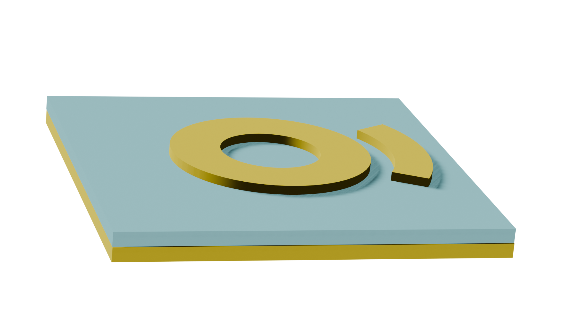
2.2 Waveguide Inverse-Taper Edge Coupler
To couple the laser output into the SiN waveguide, the chip is placed directly
at the laser edge and the SiN entrance is narrowed into an inverse taper. The
complex laser-output field stored in data/sim_data.hdf5 computed from the laser cavity portion of the notebook is replayed as a
Tidy3D CustomFieldSource. A 2D effective-index FDTD sweep then varies taper
tip width and taper length to maximize fundamental-mode coupling while limiting
reflection.
The complete sweep construction, optional cost estimate/cloud run, HDF5 result reader, and plotting workflow are contained below. The cloud sweep runs only if its results are not already saved on disk; otherwise the saved results are reused.
This next codeblock was written to deal with folder and location data issues. If you are running everything in the same folder/directory, we imagine this portion will need to be changed slightly, and can likely be omitted to a degree.
import json
from dataclasses import asdict, dataclass
from pathlib import Path

import matplotlib.pyplot as plt
import numpy as np
import tidy3d as td
import tidy3d.web as web


def _inverse_taper_find_path(*relative_candidates):
    """Find the first existing candidate path from common notebook roots.

    The fallback path is returned even when it does not exist so the calling
    function can raise a specific, user-facing ``FileNotFoundError``.
    """

    roots = [Path.cwd().resolve()]
    if "__file__" in globals():
        roots.insert(0, Path(__file__).resolve().parent)
    roots.extend(root / "final_submission" for root in tuple(roots))

    # Preserve search order while removing duplicate roots.
    roots = list(dict.fromkeys(roots))
    for root in roots:
        for relative_path in relative_candidates:
            candidate = (root / relative_path).resolve()
            if candidate.exists():
                return candidate
    return (roots[0] / relative_candidates[0]).resolve()


FINAL_SUBMISSION_ROOT = _inverse_taper_find_path("data/sim_data.hdf5").parent.parent
SIN_INVERSE_TAPER_SOURCE_HDF5 = _inverse_taper_find_path(
    "data/sim_data.hdf5",
    "final_submission/data/sim_data.hdf5",
)
SIN_INVERSE_TAPER_PASSIVE_NEFF_HDF5 = _inverse_taper_find_path(
    (
        "passive_sin_mode_sweep_fig1a_width_0020_1000_h0220_te_modes_no_si_cloud/"
        "passive_sin_mode_sweep.hdf5"
    ),
    (
        "final_submission/"
        "passive_sin_mode_sweep_fig1a_width_0020_1000_h0220_te_modes_no_si_cloud/"
        "passive_sin_mode_sweep.hdf5"
    ),
)
SIN_INVERSE_TAPER_SWEEP_DIR = (
    FINAL_SUBMISSION_ROOT / "sin_inverse_taper_2d_sweep_from_sim_data"
)
SIN_INVERSE_TAPER_ANALYSIS_DIR = SIN_INVERSE_TAPER_SWEEP_DIR / "analysis"
SIN_INVERSE_TAPER_TASK_PREFIX = "sim_data_custom_source_taper_2d"

# Point the passive-neff data at the SiN sweep result produced earlier in this notebook.
SIN_INVERSE_TAPER_PASSIVE_NEFF_HDF5 = SIN_SWEEP_HDF5
@dataclass(frozen=True)
class InverseTaperSweepConfig:
    """Settings for the 2D effective-index inverse-taper sweep."""

    wavelength_um: float = 0.740
    bus_width_um: float = 0.50
    tip_width_min_um: float = 0.05
    tip_width_max_um: float = 0.40
    tip_width_step_um: float = 0.05
    length_min_um: float = 50.0
    length_max_um: float = 500.0
    length_step_um: float = 25.0
    bus_length_um: float = 6.0
    source_gap_um: float = 0.45
    source_z_slice_um: float = 0.03
    core_neff: float = 1.78
    clad_index: float = 1.444
    sim_y_span_um: float = 4.0
    pml_padding_x_um: float = 1.2
    monitor_y_span_um: float = 3.2
    run_time_s: float = 1.2e-12
    extra_settle_time_s: float = 0.35e-12
    shutoff: float = 1e-5
    min_steps_per_wvl: float = 12.0
    num_modes: int = 4
These next functions help to load the field stored from the laser cavity simulations above.
def inverse_taper_load_json_metadata(h5):
    """Decode the JSON metadata embedded in a Tidy3D HDF5 file."""

    raw = h5["JSON_STRING"][()]
    text = raw.decode() if isinstance(raw, bytes) else str(raw)
    return json.loads(text)


def inverse_taper_monitor_index(metadata):
    """Map each simulation monitor name to its numeric HDF5 data group."""

    monitors = metadata.get("simulation", {}).get("monitors", [])
    return {monitor["name"]: index for index, monitor in enumerate(monitors)}


def inverse_taper_read_component(h5, monitor_name, component):
    """Read one complex field component and its x/y/z/f coordinates."""

    names = inverse_taper_monitor_index(inverse_taper_load_json_metadata(h5))
    if monitor_name not in names:
        raise KeyError(
            f"Monitor {monitor_name!r} not found. Available monitors: {sorted(names)}"
        )
    component_path = f"data/{names[monitor_name]}/{component}"
    if component_path not in h5:
        raise KeyError(
            f"Component {component!r} is unavailable for monitor {monitor_name!r}."
        )
    group = h5[component_path]
    values = np.asarray(group["__xarray_dataarray_variable__"])
    x = np.asarray(group["x"], dtype=float)
    y = np.asarray(group["y"], dtype=float)
    z = np.asarray(group["z"], dtype=float)
    f = np.asarray(group["f"], dtype=float)
    return values, x, y, z, f
Here, we create a function that loads the data from the hdf5 file and treats the mode as a custom source that will be placed directly at the edge of the waveguide/input coupler.
def inverse_taper_load_custom_source(
    source_hdf5,
    monitor_name,
    source_component,
    z_slice_um,
    target_wavelength_um,
    source_x_um,
):
    """Create a normalized 2D custom source from a saved laser field.

    The nearest saved wavelength and z slice are selected, then the complex
    ``source_component(y)`` profile is mapped to the 2D simulation's ``Ez``.
    """

    source_hdf5 = Path(source_hdf5)
    if not source_hdf5.exists():
        raise FileNotFoundError(f"Laser source HDF5 not found: {source_hdf5}")

    with h5py.File(source_hdf5, "r") as h5:
        values, x, y, z, f = inverse_taper_read_component(
            h5, monitor_name, source_component
        )

    expected_shape = (x.size, y.size, z.size, f.size)
    if x.size != 1 or y.size <= 1 or z.size <= 1 or values.shape != expected_shape:
        raise ValueError(
            f"Monitor {monitor_name!r} is not a replayable y-z field plane; "
            f"received {values.shape}, expected {expected_shape}."
        )

    wavelengths_um = td.C_0 / f
    frequency_index = int(np.argmin(np.abs(wavelengths_um - target_wavelength_um)))
    z_index = int(np.argmin(np.abs(z - z_slice_um)))
    # Index axes explicitly; np.squeeze would break for single-frequency data.
    lateral = np.asarray(
        values[0, :, z_index, frequency_index],
        dtype=complex,
    )
    lateral /= max(float(np.nanmax(np.abs(lateral))), 1e-30)
    freq0 = float(f[frequency_index])
    field_dataset = td.FieldDataset(
        Ez=td.ScalarFieldDataArray(
            lateral.reshape(1, y.size, 1, 1),
            coords={
                "x": [source_x_um],
                "y": y,
                "z": [0.0],
                "f": [freq0],
            },
        )
    )
    source_metadata = {
        "source_monitor": monitor_name,
        "source_component": source_component,
        "source_x_um_original": float(np.ravel(x)[0]),
        "source_z_slice_um_requested": float(z_slice_um),
        "source_z_slice_um_selected": float(z[z_index]),
        "source_wavelength_um_requested": float(target_wavelength_um),
        "source_wavelength_um_selected": float(wavelengths_um[frequency_index]),
        "source_frequency_hz": freq0,
        "source_y_min_um": float(y[0]),
        "source_y_max_um": float(y[-1]),
        "source_profile_mapping": (f"{source_component}(y,z_slice) -> 2D Ez(y)"),
    }
    return field_dataset, y, freq0, source_metadata
def inverse_taper_load_bus_neff(passive_hdf5, width_um, wavelength_um):
    """Select the fundamental TE-like effective index nearest a target point."""

    passive_hdf5 = Path(passive_hdf5)
    if not passive_hdf5.exists():
        raise FileNotFoundError(
            f"Passive SiN mode-sweep HDF5 not found: {passive_hdf5}"
        )

    with h5py.File(passive_hdf5, "r") as h5:
        widths = np.asarray(h5["width_um"], dtype=float)
        wavelengths = np.asarray(h5["wavelength_um"], dtype=float)
        neff = np.asarray(h5["n_eff_real"], dtype=float)
        te_fraction = np.asarray(h5["te_fraction"], dtype=float)
        core_fraction = np.asarray(h5["core_fraction"], dtype=float)
        height_um = float(np.asarray(h5["height_um"], dtype=float)[0])

    width_index = int(np.argmin(np.abs(widths - width_um)))
    wavelength_index = int(np.argmin(np.abs(wavelengths - wavelength_um)))
    mode_neff = neff[width_index, 0, wavelength_index, :]
    mode_te = te_fraction[width_index, 0, wavelength_index, :]
    # Prefer the highest-index mode with at least 50% TE polarization.
    te_like = np.where(mode_te >= 0.5)[0]
    if te_like.size:
        mode_index = int(te_like[np.nanargmax(mode_neff[te_like])])
    else:
        mode_index = int(np.nanargmax(mode_te))

    metadata = {
        "source_width_um": float(widths[width_index]),
        "source_height_um": height_um,
        "source_wavelength_um": float(wavelengths[wavelength_index]),
        "mode_index": float(mode_index),
        "te_fraction": float(mode_te[mode_index]),
        "core_fraction": float(
            core_fraction[width_index, 0, wavelength_index, mode_index]
        ),
    }
    return float(mode_neff[mode_index]), metadata
def inverse_taper_structure(tip_width_um, length_um, cfg):
    """Create a polygonal inverse taper followed by a straight output bus."""

    core = td.Medium(
        permittivity=cfg.core_neff**2,
        name="SiN_effective_index_core",
    )
    x0 = 0.0
    x1 = length_um
    x2 = length_um + cfg.bus_length_um
    # Traverse the lower edge forward and the upper edge backward.
    vertices = np.asarray(
        [
            (x0, -0.5 * tip_width_um),
            (x1, -0.5 * cfg.bus_width_um),
            (x2, -0.5 * cfg.bus_width_um),
            (x2, 0.5 * cfg.bus_width_um),
            (x1, 0.5 * cfg.bus_width_um),
            (x0, 0.5 * tip_width_um),
        ]
    )
    return td.Structure(
        name="sin_2d_inverse_taper",
        geometry=td.PolySlab(
            vertices=vertices,
            axis=2,
            slab_bounds=(-td.inf, td.inf),
        ),
        medium=core,
    )
Helper functions made to easily keep track of the cloud job batch.
def inverse_taper_task_name(tip_width_um, length_um):
    """Return a stable cloud task name."""

    tip_nm = int(round(1000.0 * tip_width_um))
    length_label = int(round(length_um))
    return f"{SIN_INVERSE_TAPER_TASK_PREFIX}_tip{tip_nm:03d}nm_L{length_label:03d}um"


def inverse_taper_reference_task_name():
    """Return the stable task name for the source-only normalization run."""

    return f"{SIN_INVERSE_TAPER_TASK_PREFIX}_reference_incident"


def inverse_taper_make_simulation(
    tip_width_um,
    length_um,
    cfg,
    field_dataset,
    source_y,
    freq0,
    include_taper=True,
):
    """Build one 2D FDTD taper or source-reference simulation.

    The reference case omits the taper and output monitors. Its input flux is
    used to normalize transmission, reflection, and modal coupling.
    """

    clad = td.Medium(
        permittivity=cfg.clad_index**2,
        name="SiO2_cladding",
    )
    source_x = -cfg.source_gap_um
    bus_end_x = length_um + (cfg.bus_length_um if include_taper else 0.0)
    output_x = bus_end_x - 1.0
    input_x = -0.12
    sim_x_min = source_x - cfg.pml_padding_x_um
    sim_x_max = bus_end_x + cfg.pml_padding_x_um
    sim_center_x = 0.5 * (sim_x_min + sim_x_max)
    monitor_size = (0.0, cfg.monitor_y_span_um, td.inf)
    source_size = (0.0, float(source_y[-1] - source_y[0]), td.inf)
    fwidth = freq0 / 30.0
    freqs = (freq0,)

    # Replay the saved complex laser field at the taper entrance.
    source = td.CustomFieldSource(
        name="sim_data_output_field_replay_source",
        center=(source_x, 0.0, 0.0),
        size=source_size,
        source_time=td.GaussianPulse(freq0=freq0, fwidth=fwidth),
        field_dataset=field_dataset,
    )
    mode_spec = td.ModeSpec(
        num_modes=cfg.num_modes,
        target_neff=cfg.core_neff,
        precision="double",
        sort_spec=td.ModeSortSpec(
            sort_key="n_eff",
            sort_order="descending",
            track_freq="central",
        ),
    )

    # Input monitors are shared by taper and reference simulations.
    monitors = (
        td.FluxMonitor(
            name="input_net_flux",
            center=(input_x, 0.0, 0.0),
            size=monitor_size,
            freqs=freqs,
            normal_dir="+",
        ),
        td.FluxMonitor(
            name="raw_backward_flux",
            center=(input_x, 0.0, 0.0),
            size=monitor_size,
            freqs=freqs,
            normal_dir="-",
        ),
    )
    if include_taper:
        monitors += (
            td.FluxMonitor(
                name="transmitted_flux",
                center=(output_x, 0.0, 0.0),
                size=monitor_size,
                freqs=freqs,
                normal_dir="+",
            ),
            td.ModeMonitor(
                name="bus_modes",
                center=(output_x, 0.0, 0.0),
                size=monitor_size,
                freqs=freqs,
                mode_spec=mode_spec,
                store_fields_direction="+",
            ),
        )

    # Extend runtime for pulse delay, propagation, and post-arrival settling.
    propagation_um = output_x - source_x
    source_delay_s = 5.0 / fwidth
    flight_time_s = propagation_um * cfg.core_neff / td.C_0
    run_time_s = max(
        cfg.run_time_s,
        source_delay_s + flight_time_s + cfg.extra_settle_time_s,
    )
    structures = (
        (inverse_taper_structure(tip_width_um, length_um, cfg),)
        if include_taper
        else ()
    )

    return td.Simulation(
        center=(sim_center_x, 0.0, 0.0),
        size=(sim_x_max - sim_x_min, cfg.sim_y_span_um, 0.0),
        medium=clad,
        structures=structures,
        sources=(source,),
        monitors=monitors,
        grid_spec=td.GridSpec.auto(
            wavelength=cfg.wavelength_um,
            min_steps_per_wvl=cfg.min_steps_per_wvl,
        ),
        boundary_spec=td.BoundarySpec(
            x=td.Boundary.pml(),
            y=td.Boundary.pml(),
            z=td.Boundary.periodic(),
        ),
        run_time=run_time_s,
        shutoff=cfg.shutoff,
    )
def inverse_taper_sweep_values(start, stop, step):
    """Return an inclusive floating-point sweep without dropping ``stop``."""

    return np.arange(start, stop + 0.5 * step, step)


def inverse_taper_build_sweep(cfg, source_hdf5):
    """Build the normalization run and every tip-width/length simulation."""

    field_dataset, source_y, freq0, source_metadata = inverse_taper_load_custom_source(
        source_hdf5=source_hdf5,
        monitor_name="field_yz_output",
        source_component="Ey",
        z_slice_um=cfg.source_z_slice_um,
        target_wavelength_um=cfg.wavelength_um,
        source_x_um=-cfg.source_gap_um,
    )
    simulations = {}
    rows = {}

    # The source-only run supplies the incident-flux normalization.
    reference_sim = inverse_taper_make_simulation(
        tip_width_um=cfg.bus_width_um,
        length_um=cfg.bus_length_um,
        cfg=cfg,
        field_dataset=field_dataset,
        source_y=source_y,
        freq0=freq0,
        include_taper=False,
    )
    reference_name = inverse_taper_reference_task_name()
    simulations[reference_name] = reference_sim
    rows[reference_name] = {
        "tip_width_um": float("nan"),
        "length_um": float("nan"),
        "num_cells": float(reference_sim.num_cells),
        "run_time_s": float(reference_sim.run_time),
        "is_reference": 1.0,
    }

    tip_widths = inverse_taper_sweep_values(
        cfg.tip_width_min_um,
        cfg.tip_width_max_um,
        cfg.tip_width_step_um,
    )
    lengths = inverse_taper_sweep_values(
        cfg.length_min_um,
        cfg.length_max_um,
        cfg.length_step_um,
    )
    # Generate the Cartesian product of taper-tip widths and lengths.
    for tip_width_um in tip_widths:
        for length_um in lengths:
            task_name = inverse_taper_task_name(
                float(tip_width_um),
                float(length_um),
            )
            sim = inverse_taper_make_simulation(
                tip_width_um=float(tip_width_um),
                length_um=float(length_um),
                cfg=cfg,
                field_dataset=field_dataset,
                source_y=source_y,
                freq0=freq0,
            )
            simulations[task_name] = sim
            rows[task_name] = {
                "tip_width_um": float(tip_width_um),
                "length_um": float(length_um),
                "num_cells": float(sim.num_cells),
                "run_time_s": float(sim.run_time),
                "is_reference": 0.0,
            }
    return simulations, rows, freq0, source_metadata
def inverse_taper_write_manifest(
    path,
    cfg,
    rows,
    source_metadata,
    core_neff_metadata,
):
    """Write the sweep manifest used by the embedded result reader."""

    manifest = {
        "description": (
            "2D effective-index inverse-taper sweep using sim_data.hdf5 "
            "as a CustomFieldSource"
        ),
        "source_hdf5": str(SIN_INVERSE_TAPER_SOURCE_HDF5),
        "source_metadata": source_metadata,
        "config": asdict(cfg),
        "core_neff_metadata": core_neff_metadata,
        "tasks": rows,
        "metrics_to_read": [
            "bus_modes forward mode powers / reference incident flux",
            "transmitted_flux / reference incident flux",
            "raw_backward_flux / reference incident flux",
        ],
        "caveat": (
            "This is a 2D effective-index ranking sweep. Validate selected "
            "candidates with a final 3D FDTD simulation."
        ),
        "tidy3d_version": td.__version__,
    }
    path.write_text(json.dumps(manifest, indent=2) + "\n", encoding="utf-8")
def inverse_taper_write_grid_hdf5(path, rows, cfg, source_metadata):
    """Write compact sweep-grid metadata."""

    names = list(rows)
    string_dtype = h5py.string_dtype(encoding="utf-8")
    with h5py.File(path, "w") as h5:
        h5.attrs["description"] = (
            "2D FDTD inverse-taper design grid using a custom laser source"
        )
        for key, value in asdict(cfg).items():
            h5.attrs[key] = value
        for key, value in source_metadata.items():
            h5.attrs[f"source_{key}"] = value
        h5.create_dataset(
            "task_name",
            data=np.asarray(names, dtype=object),
            dtype=string_dtype,
        )
        for field in (
            "tip_width_um",
            "length_um",
            "num_cells",
            "run_time_s",
            "is_reference",
        ):
            h5.create_dataset(
                field,
                data=np.asarray([rows[name][field] for name in names]),
            )
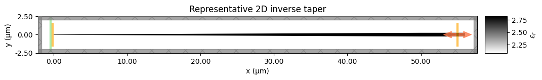
def inverse_taper_save_preview(path, sim):
    """Save a representative 2D geometry preview."""

    fig, ax = plt.subplots(figsize=(10.0, 3.8), constrained_layout=True)
    sim.plot_eps(z=0.0, ax=ax)
    ax.set_title("Representative 2D inverse taper")
    fig.savefig(path, dpi=200)
    plt.show()
def inverse_taper_prepare_batch():
    """Validate inputs, build simulations/artifacts, and return a cloud batch."""

    if not SIN_INVERSE_TAPER_SOURCE_HDF5.exists():
        raise FileNotFoundError(
            f"Laser source data not found: {SIN_INVERSE_TAPER_SOURCE_HDF5}"
        )
    if not SIN_INVERSE_TAPER_PASSIVE_NEFF_HDF5.exists():
        raise FileNotFoundError(
            "Passive SiN mode-sweep data not found: "
            f"{SIN_INVERSE_TAPER_PASSIVE_NEFF_HDF5}"
        )
    core_neff, core_neff_metadata = inverse_taper_load_bus_neff(
        SIN_INVERSE_TAPER_PASSIVE_NEFF_HDF5,
        width_um=InverseTaperSweepConfig.bus_width_um,
        wavelength_um=InverseTaperSweepConfig.wavelength_um,
    )
    cfg = InverseTaperSweepConfig(core_neff=core_neff)
    simulations, rows, freq0, source_metadata = inverse_taper_build_sweep(
        cfg,
        SIN_INVERSE_TAPER_SOURCE_HDF5,
    )

    SIN_INVERSE_TAPER_SWEEP_DIR.mkdir(parents=True, exist_ok=True)
    manifest_path = (
        SIN_INVERSE_TAPER_SWEEP_DIR
        / "sin_inverse_taper_2d_sweep_from_sim_data_manifest.json"
    )
    grid_hdf5 = (
        SIN_INVERSE_TAPER_SWEEP_DIR
        / "sin_inverse_taper_2d_sweep_from_sim_data_grid.hdf5"
    )
    batch_hdf5 = (
        SIN_INVERSE_TAPER_SWEEP_DIR
        / "sin_inverse_taper_2d_sweep_from_sim_data_batch.hdf5"
    )
    inverse_taper_write_manifest(
        manifest_path,
        cfg,
        rows,
        source_metadata,
        core_neff_metadata,
    )
    inverse_taper_write_grid_hdf5(grid_hdf5, rows, cfg, source_metadata)

    batch = web.Batch(
        simulations=simulations,
        folder_name="default",
        num_workers=10,
        verbose=True,
    )
    batch.to_file(str(batch_hdf5))

    first_taper_name = next(
        name for name, row in rows.items() if row["is_reference"] == 0.0
    )
    inverse_taper_save_preview(
        SIN_INVERSE_TAPER_SWEEP_DIR
        / "sin_inverse_taper_2d_sweep_from_sim_data_preview.png",
        simulations[first_taper_name],
    )

    cell_counts = [sim.num_cells for sim in simulations.values()]
    print(f"Built {len(simulations)} 2D FDTD simulations")
    print(f"Source HDF5: {SIN_INVERSE_TAPER_SOURCE_HDF5}")
    print("Source monitor/component: field_yz_output/Ey")
    print(
        "Selected source slice: "
        f"{1000.0 * source_metadata['source_wavelength_um_selected']:.3f} nm, "
        f"z={source_metadata['source_z_slice_um_selected']:+.4f} um"
    )
    print(f"Manifest: {manifest_path}")
    print(f"Sweep grid HDF5: {grid_hdf5}")
    print(f"Batch HDF5: {batch_hdf5}")
    print(f"2D effective core index: {cfg.core_neff:.6f}")
    print(f"Source frequency: {freq0:.6e} Hz")
    print(f"Cell count range: {min(cell_counts):,} - {max(cell_counts):,}")
    print(f"Total cells across sweep: {sum(cell_counts):,}", flush=True)
    return batch
Running the Sweep
The sweep is built and submitted to the cloud only if its results are not already present on disk; otherwise the existing results are loaded. The next cell runs the analysis once the results are available.
# Build and run the inverse-taper sweep only if its results are not already on disk.
inverse_taper_results_dir = SIN_INVERSE_TAPER_SWEEP_DIR / "results"
inverse_taper_batch = None
inverse_taper_batch_data = None
inverse_taper_batch = inverse_taper_prepare_batch()

if inverse_taper_results_dir.exists() and list(
    inverse_taper_results_dir.rglob("*.hdf5")
):
    print("Loading existing inverse-taper results from:", inverse_taper_results_dir)
else:
    inverse_taper_results_dir.mkdir(parents=True, exist_ok=True)
    inverse_taper_batch_data = inverse_taper_batch.run(
        path_dir=str(inverse_taper_results_dir)
    )
    print("Downloaded inverse-taper results to:", inverse_taper_results_dir)
Built 153 2D FDTD simulations
Source HDF5: /home/filipe/Desktop/GITHUB/tidyvernier-dual-ring-filter/tidy3d-community-library/notebooks/data/sim_data.hdf5
Source monitor/component: field_yz_output/Ey
Selected source slice: 740.253 nm, z=+0.0298 um
Manifest: /home/filipe/Desktop/GITHUB/tidyvernier-dual-ring-filter/tidy3d-community-library/notebooks/sin_inverse_taper_2d_sweep_from_sim_data/sin_inverse_taper_2d_sweep_from_sim_data_manifest.json
Sweep grid HDF5: /home/filipe/Desktop/GITHUB/tidyvernier-dual-ring-filter/tidy3d-community-library/notebooks/sin_inverse_taper_2d_sweep_from_sim_data/sin_inverse_taper_2d_sweep_from_sim_data_grid.hdf5
Batch HDF5: /home/filipe/Desktop/GITHUB/tidyvernier-dual-ring-filter/tidy3d-community-library/notebooks/sin_inverse_taper_2d_sweep_from_sim_data/sin_inverse_taper_2d_sweep_from_sim_data_batch.hdf5
2D effective core index: 1.679251
Source frequency: 4.049864e+14 Hz
Cell count range: 27,376 - 1,692,262
Total cells across sweep: 143,639,920
Loading existing inverse-taper results from: /home/filipe/Desktop/GITHUB/tidyvernier-dual-ring-filter/tidy3d-community-library/notebooks/sin_inverse_taper_2d_sweep_from_sim_data/results
INVERSE_TAPER_C_UM_PER_S = 299_792_458.0 * 1e6


def inverse_taper_wavelength_um(freq_hz):
    """Convert frequency in Hz to wavelength in micrometers."""

    return INVERSE_TAPER_C_UM_PER_S / np.asarray(freq_hz, dtype=float)
Helper functions to get the names stored in the cloud.
def inverse_taper_load_batch_task_map(batch_hdf5):
    """Return task-id to task-name mapping from a Tidy3D batch HDF5."""

    if not batch_hdf5.exists():
        return {}
    with h5py.File(batch_hdf5, "r") as h5:
        if "JSON_STRING" not in h5:
            return {}
        metadata = inverse_taper_load_json_metadata(h5)
    mapping = {}
    for task_name, job in metadata.get("jobs_cached", {}).items():
        task_id = job.get("task_id_cached")
        if task_id:
            mapping[str(task_id)] = str(task_name)
    return mapping


def inverse_taper_find_result_files(results_dir):
    """Find downloaded raw Tidy3D result files."""

    return sorted(
        path
        for path in results_dir.rglob("*.hdf5")
        if path.name != "batch.hdf5"
        and "analysis" not in path.parts
        and "sweep_grid" not in path.name
        and "sweep_batch" not in path.name
    )
Taking the online data and storing it as hdf5 files.
def inverse_taper_task_from_path(path, task_rows):
    """Infer a manifest task name from a downloaded result path."""

    task_id_map = inverse_taper_load_batch_task_map(path.parent / "batch.hdf5")
    mapped = task_id_map.get(path.stem)
    if mapped in task_rows:
        return mapped
    clean = path.stem.replace("_results", "")
    if clean in task_rows:
        return clean
    for task_name in task_rows:
        if task_name in str(path):
            return task_name
    return None


def inverse_taper_read_flux(h5, index):
    """Read frequency and values from one flux monitor."""

    group = h5[f"data/{index}/flux"]
    return (
        np.asarray(group["f"], dtype=float),
        np.asarray(
            group["__xarray_dataarray_variable__"],
            dtype=float,
        ),
    )


def inverse_taper_read_named_flux(h5, names, candidates):
    """Read the first available flux monitor in `candidates`."""

    for name in candidates:
        if name in names:
            return inverse_taper_read_flux(h5, names[name])
    raise KeyError(f"None of {candidates} found. Available monitors: {sorted(names)}")


def inverse_taper_read_mode_powers(h5, index):
    """Read forward mode powers and complex effective indices."""

    amps_group = h5[f"data/{index}/amps"]
    neff_group = h5[f"data/{index}/n_complex"]
    directions = [
        item.decode() if isinstance(item, bytes) else str(item)
        for item in np.asarray(amps_group["direction"])
    ]
    plus_index = directions.index("+")
    freqs = np.asarray(amps_group["f"], dtype=float)
    amps = np.asarray(amps_group["__xarray_dataarray_variable__"])[plus_index, :, :]
    powers = np.abs(amps) ** 2
    neff = np.asarray(neff_group["__xarray_dataarray_variable__"])
    return freqs, powers, neff


def inverse_taper_analyze_reference(path):
    """Read the source-only reference incident flux."""

    with h5py.File(path, "r") as h5:
        names = inverse_taper_monitor_index(inverse_taper_load_json_metadata(h5))
        frequencies, input_flux = inverse_taper_read_named_flux(
            h5,
            names,
            ("input_net_flux", "incident_flux"),
        )
        _, backward_flux = inverse_taper_read_named_flux(
            h5,
            names,
            ("raw_backward_flux", "reflected_flux"),
        )
    return {
        "wavelength_um": float(inverse_taper_wavelength_um(frequencies)[0]),
        "incident_reference_flux": float(np.asarray(input_flux).reshape(-1)[0]),
        "reference_raw_backward_flux": float(np.asarray(backward_flux).reshape(-1)[0]),
    }


def inverse_taper_analyze_result(path, task_row, incident_reference_flux):
    """Compute coupling, transmission, and reflection for one taper."""

    with h5py.File(path, "r") as h5:
        names = inverse_taper_monitor_index(inverse_taper_load_json_metadata(h5))
        _, input_flux = inverse_taper_read_named_flux(
            h5,
            names,
            ("input_net_flux", "incident_flux"),
        )
        _, raw_backward_flux = inverse_taper_read_named_flux(
            h5,
            names,
            ("raw_backward_flux", "reflected_flux"),
        )
        _, transmitted_flux = inverse_taper_read_named_flux(
            h5,
            names,
            ("transmitted_flux",),
        )
        mode_frequencies, mode_powers, neff = inverse_taper_read_mode_powers(
            h5, names["bus_modes"]
        )

    input_net = float(np.asarray(input_flux).reshape(-1)[0])
    raw_backward = float(np.asarray(raw_backward_flux).reshape(-1)[0])
    transmitted = float(np.asarray(transmitted_flux).reshape(-1)[0])
    powers = np.asarray(mode_powers, dtype=float).reshape(-1)
    guided_sum = float(np.sum(powers))
    incident = (
        incident_reference_flux if incident_reference_flux is not None else input_net
    )
    reflectance = (incident - input_net) / incident if incident else float("nan")
    if np.isfinite(reflectance):
        reflectance = float(np.clip(reflectance, 0.0, 1.0))

    return {
        "tip_width_um": float(task_row["tip_width_um"]),
        "length_um": float(task_row["length_um"]),
        "num_cells": float(task_row["num_cells"]),
        "run_time_s": float(task_row.get("run_time_s", float("nan"))),
        "wavelength_um": float(inverse_taper_wavelength_um(mode_frequencies)[0]),
        "incident_reference_flux": float(incident),
        "input_net_flux": input_net,
        "raw_backward_flux": raw_backward,
        "transmitted_flux": transmitted,
        "transmittance": (transmitted / incident if incident else float("nan")),
        "reflectance": reflectance,
        "flux_out_over_flux_in": (
            transmitted / input_net if input_net else float("nan")
        ),
        "guided_power_sum": guided_sum,
        "guided_over_incident": (guided_sum / incident if incident else float("nan")),
        "guided_over_flux_in": (guided_sum / input_net if input_net else float("nan")),
        "mode0_power": (float(powers[0]) if powers.size > 0 else float("nan")),
        "mode1_power": (float(powers[1]) if powers.size > 1 else float("nan")),
        "mode2_power": (float(powers[2]) if powers.size > 2 else float("nan")),
        "mode0_coupling_efficiency": (
            float(powers[0] / incident)
            if incident and powers.size > 0
            else float("nan")
        ),
        "mode1_coupling_efficiency": (
            float(powers[1] / incident)
            if incident and powers.size > 1
            else float("nan")
        ),
        "mode2_coupling_efficiency": (
            float(powers[2] / incident)
            if incident and powers.size > 2
            else float("nan")
        ),
        "mode0_over_flux_in": (
            float(powers[0] / input_net)
            if input_net and powers.size > 0
            else float("nan")
        ),
        "mode0_guided_fraction": (
            float(powers[0] / guided_sum)
            if guided_sum and powers.size > 0
            else float("nan")
        ),
        "mode0_neff_real": (
            float(np.real(neff.reshape(-1)[0])) if neff.size else float("nan")
        ),
        "mode0_neff_imag": (
            float(np.imag(neff.reshape(-1)[0])) if neff.size else float("nan")
        ),
    }


def inverse_taper_metric_grid(rows, metric):
    """Return tip, length, and metric arrays for a heatmap."""

    tips = np.asarray(sorted({row["tip_width_um"] for row in rows}))
    lengths = np.asarray(sorted({row["length_um"] for row in rows}))
    grid = np.full((lengths.size, tips.size), np.nan)
    tip_index = {value: index for index, value in enumerate(tips)}
    length_index = {value: index for index, value in enumerate(lengths)}
    for row in rows:
        grid[
            length_index[row["length_um"]],
            tip_index[row["tip_width_um"]],
        ] = row[metric]
    return tips, lengths, grid


def inverse_taper_write_analysis_hdf5(path, rows, manifest):
    """Write all scalar taper metrics to a compact HDF5 file."""

    with h5py.File(path, "w") as h5:
        h5.attrs["description"] = (
            "2D FDTD inverse-taper metrics from the laser custom source"
        )
        h5.attrs["source_hdf5"] = manifest.get("source_hdf5", "")
        for key, value in manifest.get("source_metadata", {}).items():
            h5.attrs[f"source_{key}"] = value
        for field in rows[0]:
            h5.create_dataset(
                field,
                data=np.asarray([row[field] for row in rows], dtype=float),
            )
Plots the source amplitude and height adjusted maxima.
def inverse_taper_plot_source(path, manifest):
    """Plot the source-plane intensity and selected replay slice."""

    source_hdf5 = Path(manifest["source_hdf5"])
    metadata = manifest["source_metadata"]
    monitor_name = str(metadata["source_monitor"])
    component = str(metadata["source_component"])
    selected_wavelength_um = float(metadata["source_wavelength_um_selected"])
    selected_z_um = float(metadata["source_z_slice_um_selected"])

    with h5py.File(source_hdf5, "r") as h5:
        values, _, y, z, frequencies = inverse_taper_read_component(
            h5,
            monitor_name,
            component,
        )

    wavelengths = inverse_taper_wavelength_um(frequencies)
    frequency_index = int(np.argmin(np.abs(wavelengths - selected_wavelength_um)))
    z_index = int(np.argmin(np.abs(z - selected_z_um)))
    field = np.squeeze(values)[:, :, frequency_index]
    intensity = np.abs(field) ** 2
    intensity /= max(float(np.nanmax(intensity)), 1e-30)

    fig, axes = plt.subplots(
        1,
        2,
        figsize=(11.2, 4.2),
        constrained_layout=True,
    )
    image = axes[0].imshow(
        intensity.T,
        origin="lower",
        extent=(
            float(y[0]),
            float(y[-1]),
            float(z[0]),
            float(z[-1]),
        ),
        aspect="auto",
        cmap="magma",
    )
    axes[0].axhline(
        float(z[z_index]),
        color="white",
        linewidth=1.2,
        alpha=0.85,
    )
    axes[0].set_xlabel("y [um]")
    axes[0].set_ylabel("z [um]")
    axes[0].set_title(
        f"source |{component}|^2 at {1000.0 * wavelengths[frequency_index]:.2f} nm"
    )
    fig.colorbar(image, ax=axes[0], label="normalized intensity")

    axes[1].plot(y, intensity[:, z_index], linewidth=2.0)
    axes[1].set_xlabel("y [um]")
    axes[1].set_ylabel("normalized |field|^2")
    axes[1].set_title(f"replayed lateral slice, z={z[z_index]:+.4f} um")
    axes[1].grid(True, alpha=0.3)
    fig.savefig(path, dpi=220)
    plt.show()
Plotting functions used to characterize and validate the sweep.
def inverse_taper_plot_heatmaps(path, rows):
    """Plot coupling, throughput, transmission, and reflection heatmaps."""

    metrics = [
        ("mode0_coupling_efficiency", "TE0 coupling / incident", "viridis"),
        ("flux_out_over_flux_in", "flux_out / flux_in", "viridis"),
        ("transmittance", "transmittance", "viridis"),
        ("reflectance", "reflectance", "magma"),
    ]
    fig, axes = plt.subplots(
        1,
        4,
        figsize=(17.2, 4.2),
        constrained_layout=True,
    )
    for ax, (metric, title, cmap) in zip(axes, metrics):
        tips, lengths, grid = inverse_taper_metric_grid(rows, metric)
        image = ax.imshow(
            grid,
            origin="lower",
            extent=(
                float(tips[0]),
                float(tips[-1]),
                float(lengths[0]),
                float(lengths[-1]),
            ),
            aspect="auto",
            cmap=cmap,
        )
        ax.set_xlabel("tip width [um]")
        ax.set_ylabel("length [um]")
        ax.set_title(title)
        fig.colorbar(image, ax=ax)
    fig.savefig(path, dpi=220)
    plt.show()


def inverse_taper_plot_tradeoffs(path, rows):
    """Plot coupling/reflection tradeoffs and length trends."""

    fig, axes = plt.subplots(
        1,
        2,
        figsize=(11.6, 4.6),
        constrained_layout=True,
    )
    scatter = axes[0].scatter(
        [row["reflectance"] for row in rows],
        [row["mode0_coupling_efficiency"] for row in rows],
        c=[row["length_um"] for row in rows],
        s=46,
        cmap="viridis",
    )
    axes[0].set_xlabel("reflectance")
    axes[0].set_ylabel("TE0 coupling / incident")
    axes[0].set_title("coupling vs reflection")
    axes[0].grid(True, alpha=0.3)
    fig.colorbar(scatter, ax=axes[0], label="length [um]")

    tips, _, _ = inverse_taper_metric_grid(
        rows,
        "flux_out_over_flux_in",
    )
    for tip in tips:
        tip_rows = sorted(
            (row for row in rows if row["tip_width_um"] == tip),
            key=lambda row: row["length_um"],
        )
        axes[1].plot(
            [row["length_um"] for row in tip_rows],
            [row["flux_out_over_flux_in"] for row in tip_rows],
            marker="o",
            linewidth=1.4,
            markersize=3.2,
            label=f"{tip:.2f} um",
        )
    axes[1].set_xlabel("length [um]")
    axes[1].set_ylabel("flux_out / flux_in")
    axes[1].set_title("direct throughput vs taper length")
    axes[1].grid(True, alpha=0.3)
    axes[1].legend(title="tip", fontsize=7, ncols=2)
    fig.savefig(path, dpi=220)
    plt.show()
Creates a markdown file that can be used to rank the choice of input coupler.
def inverse_taper_write_summary(path, rows, analysis_hdf5):
    """Write a Markdown table of the highest-performing candidates."""

    score = lambda row: row["mode0_coupling_efficiency"] - 0.25 * row["reflectance"]
    best = max(rows, key=score)
    best_flux = max(rows, key=lambda row: row["flux_out_over_flux_in"])
    ranked = sorted(rows, key=score, reverse=True)
    ranked_flux = sorted(
        rows,
        key=lambda row: row["flux_out_over_flux_in"],
        reverse=True,
    )
    lines = [
        "# Sim-Data Custom-Source Inverse Taper Sweep",
        "",
        f"- Designs analyzed: `{len(rows)}`",
        (
            "- Best balanced candidate: "
            f"tip `{best['tip_width_um']:.3f} um`, "
            f"length `{best['length_um']:.1f} um`"
        ),
        (f"- TE0 coupling / incident: `{best['mode0_coupling_efficiency']:.4f}`"),
        (
            "- Direct flux efficiency flux_out/flux_in: "
            f"`{best['flux_out_over_flux_in']:.4f}`"
        ),
        f"- Transmittance: `{best['transmittance']:.4f}`",
        f"- Reflectance: `{best['reflectance']:.4f}`",
        (
            "- Best direct flux candidate: "
            f"tip `{best_flux['tip_width_um']:.3f} um`, "
            f"length `{best_flux['length_um']:.1f} um`, "
            f"flux_out/flux_in "
            f"`{best_flux['flux_out_over_flux_in']:.4f}`"
        ),
        "",
        f"Processed HDF5: `{analysis_hdf5}`",
        "",
        "## Top Balanced Candidates",
        "",
        (
            "| rank | tip width | length | TE0 coupling | "
            "flux_out/flux_in | transmittance | reflectance | "
            "TE0 guided fraction |"
        ),
        "|---:|---:|---:|---:|---:|---:|---:|---:|",
    ]
    for rank, row in enumerate(ranked[:12], start=1):
        lines.append(
            f"| {rank} | {row['tip_width_um']:.3f} um | "
            f"{row['length_um']:.1f} um | "
            f"{row['mode0_coupling_efficiency']:.4f} | "
            f"{row['flux_out_over_flux_in']:.4f} | "
            f"{row['transmittance']:.4f} | "
            f"{row['reflectance']:.4f} | "
            f"{row['mode0_guided_fraction']:.4f} |"
        )
    lines.extend(
        [
            "",
            "## Top Direct Flux Candidates",
            "",
            (
                "| rank | tip width | length | flux_out/flux_in | "
                "TE0 coupling | reflectance |"
            ),
            "|---:|---:|---:|---:|---:|---:|",
        ]
    )
    for rank, row in enumerate(ranked_flux[:12], start=1):
        lines.append(
            f"| {rank} | {row['tip_width_um']:.3f} um | "
            f"{row['length_um']:.1f} um | "
            f"{row['flux_out_over_flux_in']:.4f} | "
            f"{row['mode0_coupling_efficiency']:.4f} | "
            f"{row['reflectance']:.4f} |"
        )
    path.write_text("\n".join(lines) + "\n", encoding="utf-8")
This is the main function that plots all of the outputs from the file sweep.
def inverse_taper_analyze_sweep():
    """Read downloaded results and generate all inverse-taper outputs."""

    manifest_path = (
        SIN_INVERSE_TAPER_SWEEP_DIR
        / "sin_inverse_taper_2d_sweep_from_sim_data_manifest.json"
    )
    results_dir = SIN_INVERSE_TAPER_SWEEP_DIR / "results"
    SIN_INVERSE_TAPER_ANALYSIS_DIR.mkdir(parents=True, exist_ok=True)

    manifest = json.loads(manifest_path.read_text(encoding="utf-8"))
    task_rows = manifest["tasks"]
    task_to_result = {}
    skipped = []
    for result_path in inverse_taper_find_result_files(results_dir):
        task_name = inverse_taper_task_from_path(result_path, task_rows)
        if task_name is None:
            skipped.append(result_path)
        else:
            task_to_result[task_name] = result_path

    reference_tasks = [
        task_name
        for task_name, row in task_rows.items()
        if float(row.get("is_reference", 0.0)) > 0.5
    ]
    incident_reference_flux = None
    if reference_tasks:
        reference_task = reference_tasks[0]
        if reference_task not in task_to_result:
            raise RuntimeError(
                f"Reference task {reference_task!r} is missing from {results_dir}."
            )
        incident_reference_flux = inverse_taper_analyze_reference(
            task_to_result[reference_task]
        )["incident_reference_flux"]

    rows = []
    for task_name, result_path in task_to_result.items():
        task_row = task_rows[task_name]
        if float(task_row.get("is_reference", 0.0)) > 0.5:
            continue
        rows.append(
            inverse_taper_analyze_result(
                result_path,
                task_row,
                incident_reference_flux,
            )
        )
    if not rows:
        raise RuntimeError(
            f"No matching inverse-taper result HDF5 files found in {results_dir}."
        )
    rows = sorted(
        rows,
        key=lambda row: (row["tip_width_um"], row["length_um"]),
    )

    inverse_taper_write_analysis_hdf5(
        SIN_INVERSE_TAPER_ANALYSIS_HDF5,
        rows,
        manifest,
    )
    inverse_taper_plot_source(
        SIN_INVERSE_TAPER_SOURCE_PNG,
        manifest,
    )
    inverse_taper_plot_heatmaps(
        SIN_INVERSE_TAPER_HEATMAPS_PNG,
        rows,
    )
    inverse_taper_plot_tradeoffs(
        SIN_INVERSE_TAPER_TRADEOFFS_PNG,
        rows,
    )
    inverse_taper_write_summary(
        SIN_INVERSE_TAPER_SUMMARY_MD,
        rows,
        SIN_INVERSE_TAPER_ANALYSIS_HDF5,
    )

    best = max(
        rows,
        key=lambda row: row["mode0_coupling_efficiency"] - 0.25 * row["reflectance"],
    )
    print(f"Analyzed {len(rows)} inverse-taper result files")
    print(
        "Best balanced candidate: "
        f"tip={best['tip_width_um']:.3f} um, "
        f"L={best['length_um']:.1f} um, "
        f"TE0={best['mode0_coupling_efficiency']:.4f}, "
        f"flux_out/flux_in={best['flux_out_over_flux_in']:.4f}, "
        f"T={best['transmittance']:.4f}, "
        f"R={best['reflectance']:.4f}"
    )
    if skipped:
        print(f"Skipped {len(skipped)} unmatched HDF5 files")
    return rows


SIN_INVERSE_TAPER_ANALYSIS_HDF5 = (
    SIN_INVERSE_TAPER_ANALYSIS_DIR
    / "sin_inverse_taper_2d_sweep_from_sim_data_analysis.hdf5"
)
SIN_INVERSE_TAPER_SOURCE_PNG = (
    SIN_INVERSE_TAPER_ANALYSIS_DIR / "sim_data_custom_source_profile.png"
)
SIN_INVERSE_TAPER_HEATMAPS_PNG = (
    SIN_INVERSE_TAPER_ANALYSIS_DIR
    / "sin_inverse_taper_2d_sweep_from_sim_data_heatmaps.png"
)
SIN_INVERSE_TAPER_TRADEOFFS_PNG = (
    SIN_INVERSE_TAPER_ANALYSIS_DIR
    / "sin_inverse_taper_2d_sweep_from_sim_data_tradeoffs.png"
)
SIN_INVERSE_TAPER_SUMMARY_MD = (
    SIN_INVERSE_TAPER_ANALYSIS_DIR
    / "sin_inverse_taper_2d_sweep_from_sim_data_summary.md"
)

inverse_taper_results_dir = SIN_INVERSE_TAPER_SWEEP_DIR / "results"
inverse_taper_manifest_path = (
    SIN_INVERSE_TAPER_SWEEP_DIR
    / "sin_inverse_taper_2d_sweep_from_sim_data_manifest.json"
)
if inverse_taper_results_dir.exists() and inverse_taper_manifest_path.exists():
    inverse_taper_analysis_rows = inverse_taper_analyze_sweep()
else:
    print(
        "Run the inverse-taper sweep first; no results found in",
        inverse_taper_results_dir,
    )
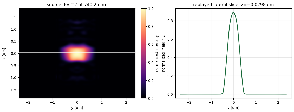
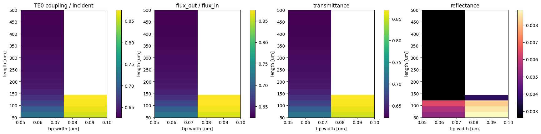
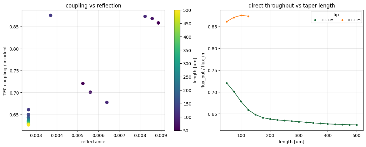
Analyzed 23 inverse-taper result files
Best balanced candidate: tip=0.100 um, L=125.0 um, TE0=0.8756, flux_out/flux_in=0.8739, T=0.8706, R=0.0037
The best input coupler has a 0.15 µm width and a 450 µm length (but for situations where space is a premium a sufficiently wide coupler with a coupler input can have similar performance at a much smaller length down to 100 µm.)
3. SiN Ring Resonator
Silicon Nitride Microring Design: Effective-Index Sweep and 3D Vernier Verification
This section demonstrates a workflow for designing silicon nitride (SiN) microring resonators in the visible / near-infrared band from 715 nm to 750 nm.
The workflow has two stages:
- Use a 2D effective-index approximation (EIA) to sweep the ring radius and bus-ring coupling gap at reduced computational cost.
- Promote two selected radii to full 3D FDTD simulations and compare their resonance combs for a Vernier pair design.
Background
A microring resonator supports circulating modes when the round-trip phase satisfies a resonance condition. The ring radius primarily controls the round-trip optical path length and therefore the free spectral range (FSR),
$$ \mathrm{FSR} \approx \frac{\lambda^2}{n_g 2\pi R}. $$
Here, $n_g$ is the group index and $R$ is the centerline radius. The bus-ring gap controls evanescent coupling, which affects the loaded quality factor, extinction, and drop efficiency.
A Vernier design uses two rings with slightly different radii. Their resonance combs have slightly different FSRs, so only selected resonances overlap. This creates a larger spectral envelope period than either ring alone, which is useful for filtering and sensing.
Imports
The notebook uses Tidy3D for FDTD simulations, the Tidy3D dispersion fitter for effective-index media, and SciPy for peak finding and lineshape fitting.
# Import the numerical, plotting, optimization, and Tidy3D APIs used throughout the notebook.
from __future__ import annotations

from dataclasses import dataclass
from pathlib import Path
import csv
import re

import matplotlib.pyplot as plt
import numpy as np
import scipy.interpolate
from scipy import signal
from scipy.optimize import curve_fit

import tidy3d as td
import tidy3d.web as web
from tidy3d.plugins.dispersion import AdvancedFastFitterParam, FastDispersionFitter
from tidy3d.plugins.mode.web import run as run_mode_solver
from tidy3d.web.api.container import BatchData

td.config.logging.level = "ERROR"
3.1 Self-Contained SiN Microring Builder
The following cell builds a 3D SiO2-clad SiN add-drop microring with two straight buses, one mode source, through/drop mode monitors, and an optional field monitor.
The geometry uses constant refractive indices over the 715-750 nm band (n_SiN = 2.0, n_SiO2 = 1.45) for a lightweight design example. Replace these with dispersive materials for a final calibrated device study.
# Define the reusable parameter container and simulation factory for a 3D SiN add-drop ring.
@dataclass(frozen=True)
class SiNMRRParams:
    """Fixed waveguide cross-section, material indices, and spectral window."""

    wg_height_um: float = 0.22  # SiN core thickness (µm)
    wg_width_um: float = 0.50  # SiN waveguide width (µm)
    lambda_min_um: float = 0.715  # start wavelength for spectra (µm)
    lambda_max_um: float = 0.750  # stop wavelength for spectra (µm)
    n_wavelengths: int = 501  # monitor frequency samples across the band
    n_sin: float = 2.0  # constant SiN index for the example
    n_sio2: float = 1.45  # constant SiO2 cladding index for the example
    run_time_s: float = 2.5e-11  # FDTD run time (s)
    min_steps_per_wvl: int = 15  # automatic mesh resolution setting
    buffer_um: float | None = None  # simulation padding; if None use _default_buffer


def _default_buffer(lambda_center_um: float) -> float:
    return float(max(0.7 * lambda_center_um, 0.45))


def build_sin_ring_mrr_sim(
    ring_radius_um: float,
    gap_um: float,
    params: SiNMRRParams | None = None,
    *,
    n_wavelengths: int | None = None,
    field_wavelengths_um: tuple[float, ...] | list[float] | None = None,
) -> td.Simulation:
    """Build a 3D SiN add-drop microring simulation.

    `ring_radius_um` is the centerline radius. `gap_um` is the edge-to-edge
    distance between ring and bus waveguides.
    """
    p = params or SiNMRRParams()
    if n_wavelengths is not None:
        p = SiNMRRParams(
            wg_height_um=p.wg_height_um,
            wg_width_um=p.wg_width_um,
            lambda_min_um=p.lambda_min_um,
            lambda_max_um=p.lambda_max_um,
            n_wavelengths=n_wavelengths,
            n_sin=p.n_sin,
            n_sio2=p.n_sio2,
            run_time_s=p.run_time_s,
            min_steps_per_wvl=p.min_steps_per_wvl,
            buffer_um=p.buffer_um,
        )

    wg_height = p.wg_height_um  # reused for all structures and port sizes
    wg_width = p.wg_width_um
    lda0 = 0.5 * (p.lambda_min_um + p.lambda_max_um)  # source center wavelength
    ldas = np.linspace(
        p.lambda_min_um, p.lambda_max_um, p.n_wavelengths
    )  # sampled wavelengths
    freqs = td.C_0 / ldas  # Tidy3D monitors are specified in frequency
    freq0 = td.C_0 / lda0  # Gaussian pulse center frequency
    fwidth = 0.5 * float(
        np.max(freqs) - np.min(freqs)
    )  # pulse bandwidth covering the sweep

    if field_wavelengths_um is None:
        field_freqs = [freq0]
    else:
        field_freqs = [td.C_0 / float(w) for w in sorted(set(field_wavelengths_um))]

    # Use simple constant-index media for this design example.
    sin = td.Medium(permittivity=p.n_sin**2)
    sio2 = td.Medium(permittivity=p.n_sio2**2)

    R = float(ring_radius_um)  # ring centerline radius (µm)
    gap = float(gap_um)  # edge-to-edge bus-ring gap (µm)
    wg_center_y = R + wg_width + gap  # bus centerline offset from ring center

    # Two straight buses form an add-drop ring: top is input/through, bottom is drop.
    waveguide_top = td.Structure(
        geometry=td.Box(center=(0, wg_center_y, 0), size=(td.inf, wg_width, wg_height)),
        medium=sin,
    )
    waveguide_bottom = td.Structure(
        geometry=td.Box(
            center=(0, -wg_center_y, 0), size=(td.inf, wg_width, wg_height)
        ),
        medium=sin,
    )

    outer = td.Cylinder(
        center=(0, 0, 0), axis=2, radius=R + wg_width / 2, length=wg_height
    )
    inner = td.Cylinder(
        center=(0, 0, 0), axis=2, radius=R - wg_width / 2, length=wg_height
    )
    ring = td.Structure(geometry=outer - inner, medium=sin)

    mode_spec = td.ModeSpec(num_modes=1, target_neff=p.n_sin)  # fundamental guided mode
    mode_plane = (
        0,
        4 * wg_width,
        6 * wg_height,
    )  # port plane spans the waveguide cross-section

    # Excite and measure the fundamental guided mode at the bus ports.
    mode_source = td.ModeSource(
        size=mode_plane,
        center=(-R, wg_center_y, 0),
        source_time=td.GaussianPulse(freq0=freq0, fwidth=fwidth),
        direction="+",
        mode_spec=mode_spec,
        mode_index=0,
        num_freqs=7,
    )
    mode_through = td.ModeMonitor(
        size=mode_plane,
        center=(R, wg_center_y, 0),
        freqs=freqs,
        mode_spec=mode_spec,
        name="through",
    )
    mode_drop = td.ModeMonitor(
        size=mode_plane,
        center=(-R, -wg_center_y, 0),
        freqs=freqs,
        mode_spec=mode_spec,
        name="drop",
    )
    field_monitor = td.FieldMonitor(
        center=(0, 0, 0),
        size=(td.inf, td.inf, 0),
        freqs=field_freqs,
        name="field",
    )

    buffer = p.buffer_um if p.buffer_um is not None else _default_buffer(lda0)
    l_x = 2 * R + wg_width + 2 * buffer
    l_y = l_x + 2 * gap + 2 * wg_width
    l_z = wg_height + 2 * buffer

    return td.Simulation(
        center=(0, 0, 0),
        size=(l_x, l_y, l_z),
        grid_spec=td.GridSpec.auto(
            min_steps_per_wvl=p.min_steps_per_wvl, wavelength=lda0
        ),
        structures=[waveguide_top, waveguide_bottom, ring],
        sources=[mode_source],
        monitors=[mode_drop, mode_through, field_monitor],
        run_time=p.run_time_s,
        boundary_spec=td.BoundarySpec(
            x=td.Boundary(
                plus=td.Absorber(num_layers=60), minus=td.Absorber(num_layers=60)
            ),
            y=td.Boundary.absorber(),
            z=td.Boundary.absorber(),
        ),
        medium=sio2,
        symmetry=(0, 0, 1),
    )


def analytic_fsr_nm(ring_radius_um: float, n_g: float, lambda_um: float) -> float:
    """Large-radius estimate FSR ~ lambda^2 / (n_g 2 pi R), returned in nm."""
    fsr_um = lambda_um**2 / (n_g * 2 * np.pi * ring_radius_um)
    return float(1000 * fsr_um)
3.2 Design Parameters
The sweep below covers radius and gap: radius controls the free spectral ranges (FSRs) and bend loss, while gap controls coupling. Because the large ring size relative to the wavelength results in many
closely packed resonances, we opted to use a Vernier configuration [1] to isolate single wavelengths from
broadband sources. By utilizing two rings with slightly different FSR, a Vernier effect
is created where feedback resonances only overlap at multiples of their individual FSRs. The two radii selected for 3D Vernier verification are 11.5 µm and 14.5 µm with a 160 nm bus-ring gap.
- Y. Liu, Z. Qiu, X. Ji, A. Bancora, G. Lihachev, J. Riemensberger, R. N. Wang, A. Voloshin, and T. J. Kippenberg, “A fully hybrid integrated erbium-based laser,” Nat. Photon., vol. 18, pp. 829–835, Aug.
# Set the global geometry, material, spectral, and sweep parameters for the study.
params = SiNMRRParams(
    wg_height_um=0.22,  # SiN core thickness in z (µm)
    wg_width_um=0.50,  # SiN bus/ring waveguide width in the xy plane (µm)
    lambda_min_um=0.715,  # lower edge of the wavelength sweep (µm)
    lambda_max_um=0.750,  # upper edge of the wavelength sweep (µm)
    n_wavelengths=501,  # frequency samples for mode monitors; increase for narrower resonances
    n_sin=2.0,  # constant SiN index used in this tutorial model
    n_sio2=1.45,  # constant SiO2 cladding index used in this tutorial model
    run_time_s=2.5e-11,  # FDTD run time; increase if resonances do not decay sufficiently
    min_steps_per_wvl=15,  # automatic mesh density control
)

lda_center = 0.5 * (
    params.lambda_min_um + params.lambda_max_um
)  # band-center wavelength

# EIA sweep grid. Reduce this list for a quick tutorial run; expand for design screening.
RING_RADII_UM = [11.5, 12.5, 13.5, 14.5]  # centerline radii (µm)
GAPS_UM = [0.15, 0.16, 0.17, 0.18]  # bus-ring edge gaps (µm)

# Shortlisted 3D candidates for Vernier comparison.
VERNIER_RADII_UM = (11.5, 14.5)  # selected radii with different FSRs
VERNIER_GAP_UM = 0.16  # 160 nm coupling gap used for both final rings
NOTCH_FIT_CENTER_UM = 0.7395  # target notch used to seed local fits
NOTCH_HALF_WIDTH_UM = 0.012  # half-width of local fitting window around target notch
N_GROUP_FOR_KAPPA2 = 2.05  # approximate group index used in κ² and loss estimates

print(f"Band: {params.lambda_min_um:.3f}-{params.lambda_max_um:.3f} µm")
print(
    f"λ0 = {lda_center:.4f} µm, cross-section = {params.wg_width_um} × {params.wg_height_um} µm"
)
print("Analytic FSR estimates with n_g=2.05:")
for R in VERNIER_RADII_UM:
    print(f"  R = {R:4.1f} µm: FSR ≈ {analytic_fsr_nm(R, 2.05, lda_center):.2f} nm")
Band: 0.715-0.750 µm
λ0 = 0.7325 µm, cross-section = 0.5 × 0.22 µm
Analytic FSR estimates with n_g=2.05:
  R = 11.5 µm: FSR ≈ 3.62 nm
  R = 14.5 µm: FSR ≈ 2.87 nm
3.3 Build and Inspect One 3D Reference Ring
The 2D EIA media are fitted once from a representative 3D reference simulation. Because all rings use the same vertical cross-section and cladding, the fitted core/background effective media can be reused across the radius-gap sweep.
# Build and plot one representative 3D ring used as the cross-section reference for EIA.
R_REF_UM = VERNIER_RADII_UM[
    0
]  # reference radius used only to define the shared vertical stack
G_REF_UM = VERNIER_GAP_UM  # same 160 nm gap as the selected 3D candidates

sim_3d_ref = build_sin_ring_mrr_sim(R_REF_UM, G_REF_UM, params=params)
wg_center_y_ref = (
    R_REF_UM + params.wg_width_um + G_REF_UM
)  # bottom-bus y coordinate magnitude

print("3D reference domain (µm):", tuple(round(x, 4) for x in sim_3d_ref.size))
print("Monitors:", [m.name for m in sim_3d_ref.monitors])

fig, ax = plt.subplots(figsize=(7, 5.5))
sim_3d_ref.plot(z=0, ax=ax)
ax.set_title(f"3D reference ring: R = {R_REF_UM} µm, gap = {G_REF_UM} µm")
ax.set_aspect("equal")
plt.tight_layout()
plt.show()

# For interactive inspection in a notebook environment:
sim_3d_ref.plot_3d()
3D reference domain (µm): (24.5255, 25.8455, 1.2455)
Monitors: ['drop', 'through', 'field']
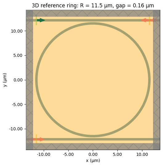
3.4 Effective-Index Approximation Helpers
This section follows the variational effective-index approach used in the Tidy3D Effective Index Approximation example. A local vertical mode solve is used to estimate an effective permittivity for the waveguide core and background. Those effective materials are then assigned to a 2D copy of the original 3D simulation.
# Define EIA utilities: vertical mode sampling, dispersive medium fitting, and 3D-to-2D conversion.
def _trapz_compat(y, x):
    """Composite trapezoid rule compatible with NumPy 1.x and 2.x."""
    y, x = np.asarray(y), np.asarray(x)
    if hasattr(np, "trapezoid"):
        return np.trapezoid(y, x=x)
    if hasattr(np, "trapz"):
        return np.trapz(y, x=x)
    import scipy.integrate as _spi

    return _spi.trapezoid(y, x=x)


def var_eps_eff(
    point, ref_point, sim, wavelength=1.55, inf=1000, min_n=1, remote=False
):
    """Variational effective permittivity at `point` relative to `ref_point`."""
    freq = td.C_0 / wavelength
    sim_2d_center = (ref_point[0], ref_point[1], 0)
    sim_2d_size = (0, inf, inf)

    # Reduce the 3D problem to a vertical slice for the slab-mode calculation.
    sim_2d = sim.updated_copy(
        center=sim_2d_center,
        size=sim_2d_size,
        sources=[],
        monitors=[],
        symmetry=(0, 0, 0),
        boundary_spec=sim.boundary_spec.updated_copy(x=td.Boundary.periodic()),
    )

    mode_solver_plane = td.Box(center=sim_2d.center, size=(td.inf, 0, td.inf))
    mode_solver = td.plugins.mode.ModeSolver(
        simulation=sim_2d,
        plane=mode_solver_plane,
        mode_spec=td.ModeSpec(num_modes=1),
        freqs=[freq],
    )
    mode_data_ref = run_mode_solver(mode_solver) if remote else mode_solver.solve()

    n_eff = mode_data_ref.n_eff.item()
    if point == ref_point:
        return n_eff**2

    x, y = ref_point
    eps_ref = sim.epsilon(
        box=td.Box(center=(x, y, sim.center[2]), size=(0, 0, td.inf)), freq=freq
    )

    x, y = point
    eps = sim.epsilon(
        box=td.Box(center=(x, y, sim.center[2]), size=(0, 0, td.inf)), freq=freq
    )

    eps_dif = np.squeeze(eps.values) - np.squeeze(eps_ref.values)
    z_coords = eps_ref.z.values
    mode_profile = mode_data_ref.Ex
    Mz2 = scipy.interpolate.interp1d(
        x=mode_profile.z.values,
        y=np.abs(np.squeeze(mode_profile.values)) ** 2,
        bounds_error=False,
        fill_value=0.0,
    )
    m_values = Mz2(z_coords)

    num = _trapz_compat(eps_dif * m_values, z_coords)
    denom = _trapz_compat(m_values, z_coords)
    if denom == 0:
        return max(n_eff**2, min_n)
    return max(n_eff**2 + num / denom, min_n)


def approximate_material(
    sim_3d, approx_point, ref_point, spectrum, min_n=1, plot=False, **fit_kwargs
):
    """Fit a dispersive medium to effective-index samples across `spectrum` in µm."""
    eps = [
        var_eps_eff(approx_point, ref_point, sim_3d, wavelength=wl, min_n=min_n)
        for wl in spectrum
    ]
    e1, e2 = np.real(eps), np.imag(eps)
    n = np.sqrt((np.sqrt(e1**2 + e2**2) + e1) / 2)
    k = np.sqrt((np.sqrt(e1**2 + e2**2) - e1) / 2)

    fitter = FastDispersionFitter(wvl_um=spectrum, n_data=n, k_data=k)
    fit_kwargs.setdefault("min_num_poles", 1)
    medium, rms_error = fitter.fit(**fit_kwargs)
    print(f"Fitted medium at {approx_point}: RMS error = {rms_error:.3e}")

    if plot:
        fig, ax = plt.subplots(figsize=(4, 3))
        fitter.plot(medium, ax=ax)
        ax.set_title("Fitted effective medium")
        plt.tight_layout()
        plt.show()
    return medium


def create_2d_sim(sim_3d, core_medium, background_medium):
    """Collapse a 3D ring simulation into a 2D EIA simulation."""
    new_structures = [s.updated_copy(medium=core_medium) for s in sim_3d.structures]
    new_size = list(sim_3d.size)
    new_size[2] = 0
    return sim_3d.updated_copy(
        size=new_size,
        structures=new_structures,
        boundary_spec=sim_3d.boundary_spec.updated_copy(z=td.Boundary.periodic()),
        medium=background_medium,
        symmetry=(0, 0, 0),
    )
3.5 Fit Effective Media Once
The reference point is placed on the bottom bus waveguide center. The background point is placed at the ring center, where the add-drop ring geometry is SiO2 cladding. The fitted media are reused for all rings in the 2D radius-gap sweep.
This step uses the local Tidy3D mode solver for the vertical slice calculations, so it does not submit a cloud FDTD task.
# Choose core/background sampling points and optionally fit the EIA media.
reference_point = (
    0.0,
    -wg_center_y_ref,
)  # point on the bottom bus core, used as EIA reference
waveguide_point = reference_point  # fitted core medium samples the same waveguide point
background_point = (0.0, 0.0)  # ring center is SiO2 background in this annular geometry

spectrum_fit_um = np.linspace(
    0.65, 0.80, 71
)  # wider fitting band than the simulation band
fit_param = AdvancedFastFitterParam(num_iters=100)  # fitter iteration budget

# Set FIT_EIA_MEDIA = True to perform local mode solves and material fitting.
# Keep False when reading pre-computed results or reviewing the notebook.
FIT_EIA_MEDIA = True  # local mode solves only; no cloud FDTD run is submitted here

if FIT_EIA_MEDIA:
    ring_waveguide_medium = approximate_material(
        sim_3d_ref,
        waveguide_point,
        reference_point,
        spectrum_fit_um,
        plot=True,
        advanced_param=fit_param,
    )
    ring_background_medium = approximate_material(
        sim_3d_ref,
        background_point,
        reference_point,
        spectrum_fit_um,
        plot=True,
        advanced_param=fit_param,
    )
    sim_2d_ref = create_2d_sim(
        sim_3d_ref, ring_waveguide_medium, ring_background_medium
    )

    fig, ax = plt.subplots(figsize=(6, 5))
    sim_2d_ref.plot_eps(z=0, freq=td.C_0 / lda_center, ax=ax)
    ax.set_title("2D EIA reference: effective permittivity")
    ax.set_aspect("equal")
    plt.tight_layout()
    plt.show()
else:
    print("Set FIT_EIA_MEDIA = True to fit EIA materials and create sim_2d_ref.")
Output()
Fitted medium at (0.0, -12.16): RMS error = 2.453e-04
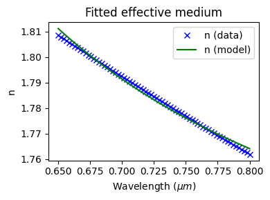
Output()
Fitted medium at (0.0, 0.0): RMS error = 1.160e-05
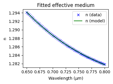
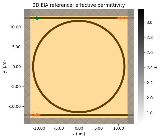
3.6 Build the 2D Radius-Gap Sweep
After fitting ring_waveguide_medium and ring_background_medium, this cell builds one 2D EIA simulation per $(R, g)$ point. Cost estimation and cloud execution are separated so that the notebook can be reviewed without launching jobs.
# Build and run the 2D EIA sweep only if the batch results are not already on disk.
EIA_BATCH_DIR = (
    Path("results") / "sin_mrr_eia_batch"
)  # where 2D batch results / CSV files are stored
sims_2d = {}
batch_2d = None  # populated only if a new run is needed
estimated_cost_2d = None  # populated by Batch.estimate_cost before running
batch_data_2d = None  # populated by the run, or loaded from disk in a later cell

if (EIA_BATCH_DIR / "batch.hdf5").exists():
    print("Loading existing 2D EIA sweep results from:", EIA_BATCH_DIR)
elif "ring_waveguide_medium" in globals() and "ring_background_medium" in globals():
    for R in RING_RADII_UM:
        for g in GAPS_UM:
            name = f"sin_mrr_R{R:g}_g{g:g}"
            sim3 = build_sin_ring_mrr_sim(R, g, params=params)
            sims_2d[name] = create_2d_sim(
                sim3, ring_waveguide_medium, ring_background_medium
            )
    print(f"Built {len(sims_2d)} 2D EIA simulations.")

    # Estimate the sweep cost before running. This does not time-step the FDTD
    # simulation, but it can create cloud task records.
    batch_2d = web.Batch(simulations=sims_2d, folder_name="sin_mrr_eia_sweep")
    estimated_cost_2d = batch_2d.estimate_cost(verbose=True)
    print("Estimated maximum FlexCredits for the full 2D EIA sweep:", estimated_cost_2d)

    EIA_BATCH_DIR.mkdir(parents=True, exist_ok=True)
    batch_data_2d = batch_2d.run(path_dir=str(EIA_BATCH_DIR))
    print(batch_data_2d.task_ids)
else:
    print(
        "EIA media not available. Run the previous cell with FIT_EIA_MEDIA = True first."
    )
Built 16 2D EIA simulations.
16:45:41 -03 Maximum FlexCredit cost: 6.194 for the whole batch.
Output()
Estimated maximum FlexCredits for the full 2D EIA sweep: 6.193551554492421
16:45:42 -03 Started working on Batch containing 16 tasks.
16:46:10 -03 Maximum FlexCredit cost: 6.194 for the whole batch.
             Use 'Batch.real_cost()' to get the billed FlexCredit cost after
             completion.
Output()
16:53:33 -03 Batch complete.
{'sin_mrr_R11.5_g0.15': 'fdve-3979a34c-b963-4d00-8c84-63dcddda9fa0', 'sin_mrr_R11.5_g0.16': 'fdve-fff4e9f3-3151-4ced-96ee-7dfd09925b90', 'sin_mrr_R11.5_g0.17': 'fdve-6781e55c-8df3-4ead-b408-be5a0e3b8ef0', 'sin_mrr_R11.5_g0.18': 'fdve-a33c153e-ce58-4850-8b49-d151ba331b31', 'sin_mrr_R12.5_g0.15': 'fdve-db601b96-2611-4f71-a84c-16bbca0f7948', 'sin_mrr_R12.5_g0.16': 'fdve-a8133221-3eed-4a6d-b806-17c63331eec5', 'sin_mrr_R12.5_g0.17': 'fdve-3ff9b2c6-2829-4db9-9fb4-284c4b5e81ed', 'sin_mrr_R12.5_g0.18': 'fdve-98f46d28-394b-4a6b-bd42-08ed2b751fc0', 'sin_mrr_R13.5_g0.15': 'fdve-a8700d22-0065-4c56-848a-099e94deba57', 'sin_mrr_R13.5_g0.16': 'fdve-88ec04aa-0ffd-485c-b1ca-94abd46f7078', 'sin_mrr_R13.5_g0.17': 'fdve-450b0c01-b3df-4e58-a16d-60561182100f', 'sin_mrr_R13.5_g0.18': 'fdve-845cdbb3-e4f1-459b-b046-fb9e935ab2e1', 'sin_mrr_R14.5_g0.15': 'fdve-8a48ed72-9b22-4ac5-af8d-30546b7046d5', 'sin_mrr_R14.5_g0.16': 'fdve-02d24e7f-7c20-43aa-8225-02bb09ae18b3', 'sin_mrr_R14.5_g0.17': 'fdve-d5ea72d8-1680-4130-9343-d63c94fbf352', 'sin_mrr_R14.5_g0.18': 'fdve-9a7dead4-6c4e-4a0a-b58e-101aa19d43a3'}
3.7 Spectra Extraction and Metrics
The same helpers work for 2D EIA and 3D SimulationData. The through monitor is read in the forward direction, while the drop monitor is read in the backward direction for this add-drop geometry.
The scalar through-notch model is used to estimate loaded quality factor, intrinsic/coupling quality factors, coupling coefficient, FSR, and loss. These estimates are intended for screening and comparison across the sweep; final values should be verified with mesh/time convergence.
Metric Equations Used in the Sweep
For each radius-gap point, the mode monitors return complex modal amplitudes. We analyze the mode power
$$ T(\lambda) = |a(\lambda)|^2. $$
The forward through monitor is used for the notch, and the backward drop monitor is used to estimate peak spacing. The through-port resonance is fit with a symmetric notch model,
$$ T_{\mathrm{thru}}(\lambda) = T_{\min} + (T_{\max} - T_{\min}) \frac{(\lambda - \lambda_0)^2}{(\lambda - \lambda_0)^2 + w^2}. $$
Here, $\lambda_0$ is the fitted resonance wavelength and $w$ is the half-width parameter. Therefore,
$$ \mathrm{FWHM} = 2w, \qquad Q_L \approx \frac{\lambda_0}{\mathrm{FWHM}}. $$
The free spectral range is estimated from adjacent drop-port peaks,
$$ \mathrm{FSR}_{\lambda} \approx \left\langle \lambda_{m+1} - \lambda_m \right\rangle, $$
and converted to an effective group index estimate through the large-radius ring relation
$$ n_g \approx \frac{\lambda_0^2}{\mathrm{FSR}_{\lambda}\,2\pi R}. $$
For the symmetric double-bus approximation, the on-resonance through power is related to the ratio $x = \Gamma_i / \Gamma_e$, where $\Gamma_i$ is the intrinsic decay rate and $\Gamma_e$ is the external decay rate into one bus:
$$ \sqrt{T_{\min}} \approx \left|\frac{x - 2}{x + 2}\right|. $$
The total decay rate is obtained from $Q_L$,
$$ \Gamma_{\mathrm{tot}} = \frac{\omega_0}{Q_L}, \qquad \Gamma_{\mathrm{tot}} = \Gamma_i + 2\Gamma_e. $$
This gives
$$ Q_i = \frac{\omega_0}{\Gamma_i}, \qquad Q_e = \frac{\omega_0}{\Gamma_e}. $$
Finally, the approximate power coupling coefficient and intrinsic loss are reported as
$$ \kappa^2 \approx \frac{n_g L}{\lambda_0 Q_e}, \qquad L = 2\pi R, $$
$$ \alpha_{\mathrm{rt}}\;[\mathrm{dB/round}] \approx \frac{10}{\ln 10}\,\Gamma_i\tau_{\mathrm{rt}}, \qquad \tau_{\mathrm{rt}} = \frac{n_g L}{c}, $$
and
$$ \alpha\;[\mathrm{dB/cm}] = \frac{\alpha_{\mathrm{rt}}}{L\;[\mathrm{cm}]}. $$
These expressions are screening metrics: they assume an isolated resonance, a scalar Lorentzian-like notch, and symmetric bus loading. Final reported values should be checked with sufficient spectral resolution, simulation runtime, and mesh convergence.
References
- Tidy3D, Ring Resonator example.
- Tidy3D, Effective Index Approximation example.
- Tidy3D, Parameter Scan / Batch example.
- B. E. Little, S. T. Chu, H. A. Haus, J. Foresi, and J.-P. Laine, “Microring resonator channel dropping filters,” Journal of Lightwave Technology 15, 998–1005 (1997).
- D. G. Rabus, Integrated Ring Resonators: The Compendium, Springer (2007).
- J. T. Smith et al., “Silicon nitride microring resonators for visible photonics,” Optical Materials Express 13, 458–470 (2023).
# Define spectral post-processing and resonator metric helpers used for both EIA and 3D data.
C_LIGHT = float(td.C_0)


def spectrum_mode_power(sim_data, monitor_name: str, direction: str):
    # Select one propagation direction from the mode monitor amplitudes.
    # For this add-drop layout: through uses direction="+"; drop uses direction="-".
    amps = sim_data[monitor_name].amps.sel(mode_index=0, direction=direction)
    f = np.asarray(amps.f.values, dtype=float)  # monitor frequencies in Hz
    wl = td.C_0 / f  # convert frequency samples to wavelength in µm (Tidy3D units)
    power = np.abs(np.asarray(amps.values, dtype=complex)) ** 2  # modal power |a|^2
    order = np.argsort(wl)  # sort by increasing wavelength for fitting and plotting
    return wl[order], power[order]


def parse_task_rg(task_name: str) -> tuple[float, float]:
    # Task names encode the sweep parameters, e.g. "sin_mrr_R11.5_g0.16".
    m = re.match(r"sin_mrr_R([0-9.]+)_g([0-9.]+)$", str(task_name))
    if not m:
        raise ValueError(f"Unexpected task name: {task_name!r}")
    return float(m.group(1)), float(m.group(2))  # radius R (µm), gap g (µm)


def coupling_regime(x: float, band: float = 0.12) -> str:
    # x = Gamma_i / Gamma_e for one bus in the symmetric double-bus model.
    # Critical through-port extinction occurs near x = 2, so we classify around that value.
    if not np.isfinite(x) or x <= 0:
        return "invalid"
    if x > 2.0 + band:
        return "undercoupled"  # intrinsic loss dominates relative to one-bus loading
    if x < 2.0 - band:
        return "overcoupled"  # external coupling dominates relative to intrinsic loss
    return "critical"  # near the through-null condition


def loss_db_per_cm(loss_db_per_round: float, R_um: float) -> float:
    # Convert round-trip loss to propagation loss by dividing by circumference in cm.
    if not np.isfinite(loss_db_per_round):
        return float("nan")
    circumference_cm = 2 * np.pi * float(R_um) * 1e-4  # µm -> cm conversion
    return float(loss_db_per_round) / circumference_cm


def _notch_seed_index(wl_um, T, prefer_lambda_um=None):
    # Choose an initial notch center for nonlinear fitting.
    wl_um, T = np.asarray(wl_um, dtype=float), np.asarray(T, dtype=float)
    if prefer_lambda_um is None or not np.isfinite(float(prefer_lambda_um)):
        return int(
            np.argmin(T)
        )  # no target wavelength: seed at the deepest through dip
    t_rng = float(np.nanmax(T) - np.nanmin(T))  # dynamic range of the trace
    prom = (
        max(1e-12, 0.015 * t_rng) if t_rng > 0 else 1e-12
    )  # small prominence threshold
    loc, _ = signal.find_peaks(
        -T, prominence=prom, distance=max(1, len(T) // 250)
    )  # dips in T
    if len(loc) == 0:
        return int(np.argmin(T))  # fallback if peak finding misses shallow notches
    return int(
        loc[int(np.argmin(np.abs(wl_um[loc] - float(prefer_lambda_um))))]
    )  # nearest local dip


def notch_through_power(wl, Tmax, Tmin, lam0, w):
    # Symmetric all-pass notch model in power. `w` is the half-width parameter in µm.
    wl = np.asarray(wl, dtype=float)
    return Tmin + (Tmax - Tmin) * (wl - lam0) ** 2 / ((wl - lam0) ** 2 + w**2)


def fit_through_notch_near(wl_um, T_through, lambda_target_um, half_width_um=0.012):
    # Restrict the fit to a target wavelength window so dense spectra do not pick the wrong notch.
    wl_um, T = np.asarray(wl_um, dtype=float), np.asarray(T_through, dtype=float)
    order = np.argsort(wl_um)
    wl_um, T = wl_um[order], T[order]

    half = float(half_width_um)  # start with the user-selected fitting half-window
    for _ in range(10):
        mask = (wl_um >= lambda_target_um - half) & (
            wl_um <= lambda_target_um + half
        )  # local fit window
        if np.count_nonzero(mask) >= 24:  # enough samples for stable nonlinear fitting
            break
        half *= 1.35  # enlarge the window if the wavelength grid is too sparse
    if np.count_nonzero(mask) >= 8:
        wl_fit, T_fit = wl_um[mask], T[mask]  # fit only near the target resonance
    else:
        wl_fit, T_fit = (
            wl_um,
            T,
        )  # fallback: use the whole spectrum if the window is undersampled

    i_min = _notch_seed_index(
        wl_fit, T_fit, lambda_target_um
    )  # initial resonance index
    lam0 = float(wl_fit[i_min])  # initial resonance wavelength
    Tmin0 = float(T_fit[i_min])  # initial notch floor
    Tmax0 = float(np.percentile(T_fit, 98))  # robust off-resonance baseline estimate
    span = float(np.max(wl_fit) - np.min(wl_fit))  # fit-domain wavelength span
    if Tmax0 <= Tmin0 + 1e-12 or span <= 0:
        return None  # invalid trace or fit window

    p0 = [Tmax0, Tmin0, lam0, max(span / 120, 1e-9)]  # initial [Tmax, Tmin, λ0, w]
    bounds = (
        [Tmin0 + 1e-9, 0.0, np.min(wl_fit), 1e-12],  # lower bounds
        [
            min(Tmax0 * 1.5 + 0.1, 10.0),
            min(Tmax0, np.max(T_fit)),
            np.max(wl_fit),
            span,
        ],  # upper bounds
    )
    try:
        popt, _ = curve_fit(
            notch_through_power, wl_fit, T_fit, p0=p0, bounds=bounds, maxfev=25000
        )
        Tmax, Tmin, l0, w = map(
            float, popt
        )  # fitted baseline, floor, center, and half-width
        if w <= 0 or Tmax <= Tmin:
            return None  # reject nonphysical fits
        return {
            "Tmax": Tmax,
            "Tmin": Tmin,
            "lam0": l0,
            "w_um": w,
            "fwhm_um": 2 * w,
        }  # FWHM = 2w
    except Exception:
        return None  # fitting can fail for flat/noisy traces


def mean_fsr_nm_from_drop_peaks(wl_um, T_drop, prominence_rel=0.04):
    # Use drop-port peaks to estimate resonance spacing in wavelength.
    wl_um, T = np.asarray(wl_um, dtype=float), np.asarray(T_drop, dtype=float)
    prom = max(
        float(prominence_rel) * (float(np.max(T)) - float(np.min(T))), 1e-12
    )  # adaptive peak prominence
    peaks, _ = signal.find_peaks(T, prominence=prom)  # drop resonances appear as peaks
    if len(peaks) < 2:
        return float("nan"), int(len(peaks))  # need at least two peaks for an FSR
    peak_wl = np.sort(wl_um[peaks])  # sort peak wavelengths before differencing
    return float(np.mean(np.diff(peak_wl)) * 1000), int(
        len(peaks)
    )  # convert µm spacing to nm


def n_g_from_fsr(lambda_um, R_um, fsr_nm):
    # Rearranged large-radius relation: FSR ≈ λ² / (n_g 2πR).
    if not np.isfinite(fsr_nm) or fsr_nm <= 0:
        return float("nan")
    fsr_um = fsr_nm / 1000  # nm -> µm to match λ and R units
    return float(lambda_um**2 / (fsr_um * 2 * np.pi * R_um))


def x_from_sqrt_Tthrough(r):
    # Invert sqrt(Tmin) ≈ |(x - 2) / (x + 2)| for x = Gamma_i / Gamma_e.
    r = float(
        np.clip(r, 0.0, 1.0 - 1e-15)
    )  # keep the algebra away from singular values
    candidates = []
    if r < 1.0 - 1e-12:
        candidates.append((2.0 + 2.0 * r) / (1.0 - r))  # branch with x > 2
    candidates.append((2.0 - 2.0 * r) / (1.0 + r))  # branch with x < 2
    best_x, best_err = np.nan, np.inf
    for x in candidates:
        if x <= 0 or not np.isfinite(x):
            continue
        err = abs(abs(x - 2.0) / (x + 2.0) - r)  # choose branch that best reproduces r
        if err < best_err:
            best_x, best_err = x, err
    return float(best_x)


def ring_metrics_row(
    task_name,
    R_um,
    gap_um,
    wl_um,
    T_drop,
    T_through,
    *,
    lambda_fit_target_um,
    notch_half_width_um=0.012,
    n_group_for_kappa2=2.05,
):
    # Combine notch fitting, FSR extraction, coupling split, and loss estimates into one table row.
    fit = fit_through_notch_near(
        wl_um, T_through, lambda_fit_target_um, half_width_um=notch_half_width_um
    )
    if fit is None:
        return {
            "task": task_name,
            "R_um": R_um,
            "gap_um": gap_um,
            "model_note": "notch_fit_failed",
        }

    lam0 = fit["lam0"]  # fitted resonance wavelength (µm)
    Q_L = (
        lam0 / fit["fwhm_um"] if fit["fwhm_um"] > 0 else float("nan")
    )  # loaded Q from linewidth
    omega0 = 2 * np.pi * (C_LIGHT / lam0)  # angular frequency in Tidy3D unit convention
    Gamma_tot = (
        omega0 / Q_L if np.isfinite(Q_L) and Q_L > 0 else float("nan")
    )  # total decay rate
    fsr_nm, n_peaks = mean_fsr_nm_from_drop_peaks(
        wl_um, T_drop
    )  # mean drop-peak spacing
    n_g_meas = n_g_from_fsr(
        lam0, R_um, fsr_nm
    )  # group index inferred from measured FSR

    Tmin_fit = float(
        np.clip(fit["Tmin"], 1e-15, 1.0)
    )  # avoid exact zero before sqrt/inversion
    x = x_from_sqrt_Tthrough(np.sqrt(Tmin_fit))  # intrinsic-to-external decay ratio

    row = {
        "task": task_name,  # original simulation / batch task name
        "R_um": R_um,  # ring centerline radius
        "gap_um": gap_um,  # bus-ring edge gap
        "lambda0_um": lam0,  # fitted through-notch center
        "fwhm_nm": 1000 * fit["fwhm_um"],  # linewidth converted from µm to nm
        "Q_loaded": Q_L,  # loaded quality factor
        "T_through_min_fit": Tmin_fit,  # fitted on-resonance through power
        "T_through_max_fit": float(fit["Tmax"]),  # fitted off-resonance through power
        "mean_fsr_nm_peaks": fsr_nm,  # mean drop peak spacing
        "n_drop_peaks": n_peaks,  # number of drop peaks used for FSR
        "n_group_from_fsr": n_g_meas,  # effective group index from FSR
        "Q_intrinsic": np.nan,  # filled after decay-rate split
        "Q_coupling": np.nan,  # filled after decay-rate split
        "kappa2_power": np.nan,  # filled after Q_e is available
        "kappa_amplitude": np.nan,  # sqrt(kappa2_power)
        "loss_dB_per_round": np.nan,  # intrinsic round-trip loss
        "loss_dB_per_cm": np.nan,  # propagation loss normalized by circumference
        "Gamma_over_Gamma_e": x,  # x = Gamma_i / Gamma_e
        "coupling_regime": "invalid",  # filled after validating x
        "model_note": "ok",  # diagnostic note for failed fits/models
    }
    if not np.isfinite(Gamma_tot) or not np.isfinite(x):
        row["model_note"] = "notch_or_split_model_failed"
        return row

    Gamma_e = Gamma_tot / (
        x + 2.0
    )  # one-bus external decay rate from Gamma_tot = Gamma_i + 2 Gamma_e
    Gamma_i = x * Gamma_e  # intrinsic decay rate
    Q_i = omega0 / Gamma_i if Gamma_i > 0 else float("nan")  # intrinsic Q
    Q_e = omega0 / Gamma_e if Gamma_e > 0 else float("nan")  # coupling Q per bus
    L_rt_um = 2 * np.pi * R_um  # ring circumference in µm
    tau_rt = n_group_for_kappa2 * L_rt_um / C_LIGHT  # approximate round-trip time
    kappa2 = (
        (n_group_for_kappa2 * L_rt_um) / (lam0 * Q_e)
        if np.isfinite(Q_e) and Q_e > 0
        else float("nan")
    )  # power coupling
    loss_rt_db = (
        (10.0 / np.log(10.0)) * Gamma_i * tau_rt if Gamma_i > 0 else float("nan")
    )  # dB per round trip

    row.update(
        Q_intrinsic=Q_i,  # intrinsic loss-limited Q
        Q_coupling=Q_e,  # external coupling Q for one bus
        kappa2_power=kappa2,  # estimated power coupling coefficient
        kappa_amplitude=float(np.sqrt(kappa2))
        if np.isfinite(kappa2) and kappa2 >= 0
        else float("nan"),
        loss_dB_per_round=loss_rt_db,  # intrinsic loss per round trip
        loss_dB_per_cm=loss_db_per_cm(loss_rt_db, R_um),  # normalized propagation loss
        coupling_regime=coupling_regime(x),  # under / critical / over-coupled label
    )
    return row
3.8 Load and Plot 2D EIA Sweep Results
If you have already run the 2D batch, place the saved batch.hdf5 directory under results/sin_mrr_eia_batch/ or set EIA_BATCH_DIR below. The cell extracts spectra, estimates FSR from drop peaks, computes notch metrics, and exports a compact CSV table.
# Load a completed 2D batch, extract spectra, compute metrics, and export a CSV summary.
def load_batch_data(path_dir: Path):
    if (path_dir / "batch.hdf5").is_file() or path_dir.is_dir():
        try:
            return BatchData.load(path_dir=str(path_dir))
        except Exception as exc:
            print(f"Could not load BatchData from {path_dir}: {exc}")
    return None


batch_data_2d = globals().get(
    "batch_data_2d", None
)  # reuse in-memory results if this kernel ran the batch
if batch_data_2d is None:
    batch_data_2d = load_batch_data(
        EIA_BATCH_DIR
    )  # otherwise try loading saved results from disk

case_results = {}  # spectra and metadata keyed by task name
# Convert each SimulationData object into sorted wavelength/power arrays for analysis.
if batch_data_2d is not None:
    for name, sim_data in batch_data_2d.items():
        R, g = parse_task_rg(name)
        wl_drop, T_drop = spectrum_mode_power(sim_data, "drop", "-")
        wl_through, T_through = spectrum_mode_power(sim_data, "through", "+")
        case_results[name] = {
            "R": R,
            "gap": g,
            "wl": wl_drop,
            "T_drop": T_drop,
            "T_through": np.interp(wl_drop, wl_through, T_through),
        }
    print(f"Loaded {len(case_results)} EIA spectra.")
else:
    print(
        "No EIA BatchData loaded. Run the batch or point EIA_BATCH_DIR to saved results."
    )

metric_rows = []  # one notch/FSR/Q/loss row per 2D sweep case
for name, d in case_results.items():
    metric_rows.append(
        ring_metrics_row(
            name,
            d["R"],
            d["gap"],
            d["wl"],
            d["T_drop"],
            d["T_through"],
            lambda_fit_target_um=NOTCH_FIT_CENTER_UM,  # choose the local notch closest to this wavelength
            notch_half_width_um=NOTCH_HALF_WIDTH_UM,  # fitting window around the target notch
            n_group_for_kappa2=N_GROUP_FOR_KAPPA2,  # approximate group index for κ² / loss conversion
        )
    )

if metric_rows:
    csv_path = EIA_BATCH_DIR / "community_eia_notch_metrics.csv"
    csv_path.parent.mkdir(parents=True, exist_ok=True)
    with csv_path.open("w", newline="") as fp:
        writer = csv.DictWriter(
            fp, fieldnames=list(metric_rows[0].keys()), extrasaction="ignore"
        )
        writer.writeheader()
        writer.writerows(metric_rows)
    print(f"Wrote {len(metric_rows)} metric rows to {csv_path}")
else:
    print("No metric rows to export.")
Loaded 16 EIA spectra.
Wrote 16 metric rows to results/sin_mrr_eia_batch/community_eia_notch_metrics.csv
# Plot representative 2D EIA spectra for the two ring radii chosen for Vernier verification.
if case_results:
    fig, ax = plt.subplots(figsize=(9, 4.5))
    for R in VERNIER_RADII_UM:
        key = f"sin_mrr_R{R:g}_g{VERNIER_GAP_UM:g}"  # matches the task naming convention used above
        if key not in case_results:
            print(f"Missing {key}")
            continue
        d = case_results[key]
        ax.plot(d["wl"], d["T_drop"], lw=1.5, label=f"R = {R:g} µm, drop")
        ax.plot(
            d["wl"],
            d["T_through"],
            ls="--",
            lw=1.1,
            alpha=0.7,
            label=f"R = {R:g} µm, through",
        )
    ax.set_xlabel("Wavelength (µm)")
    ax.set_ylabel(r"Mode power $|a|^2$")
    ax.set_title("2D EIA spectra for Vernier candidate rings")
    ax.grid(True, alpha=0.3)
    ax.legend(ncol=2, fontsize=8)
    plt.tight_layout()
    plt.show()
else:
    print("Run/load the EIA batch before plotting spectra.")
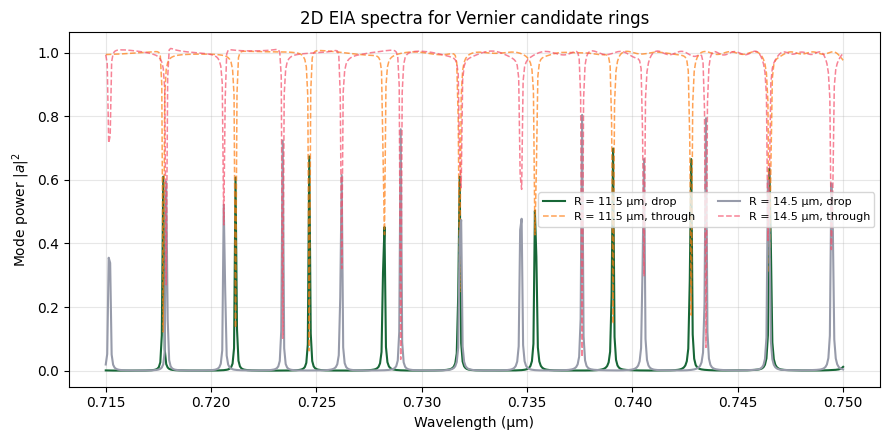
Sweep Plots at Fixed Radius and Fixed Gap
The next cell reproduces the sweep-style plots:
- Fixed radius, sweep gap: the upper panel overlays all drop/through spectra for one radius while the lower panel shows how the estimated coupling coefficient $\kappa^2$ changes with gap.
- Fixed gap, sweep radius: the upper panel overlays all drop/through spectra for one gap while the lower panel shows how the FSR changes with radius.
# Plot all sweep spectra at fixed R or fixed gap, with a metric trend in the bottom panel.
from matplotlib.collections import LineCollection
from matplotlib.colors import LinearSegmentedColormap, Normalize


def cmap_blue_violet_pink():
    # Same visual style as the development sweep notebook: blue -> violet -> pink.
    return LinearSegmentedColormap.from_list(
        "blue_violet_pink",
        ["#2563eb", "#7c3aed", "#ec4899"],
    )


def norm_span(values):
    # Normalize sweep values for color mapping; pad zero-width ranges to avoid division by zero.
    values = np.asarray(values, dtype=float)
    if values.size == 0:
        return Normalize(0.0, 1.0)
    vmin, vmax = float(np.nanmin(values)), float(np.nanmax(values))
    if np.isclose(vmin, vmax):
        pad = max(abs(vmin) * 0.05, 1e-3)
        vmin, vmax = vmin - pad, vmax + pad
    return Normalize(vmin, vmax)


def plot_metric_curve_colored(ax, x, y, *, xlabel, ylabel, title):
    # Draw a bottom-panel metric curve with the same blue-violet-pink map used for spectra.
    x = np.asarray(x, dtype=float)
    y = np.asarray(y, dtype=float)
    ok = np.isfinite(x) & np.isfinite(y)
    if np.count_nonzero(ok) == 0:
        ax.text(
            0.5, 0.5, "No finite data", ha="center", va="center", transform=ax.transAxes
        )
        ax.set_xlabel(xlabel)
        ax.set_ylabel(ylabel)
        ax.set_title(title)
        return None
    x, y = x[ok], y[ok]
    order = np.argsort(x)
    x, y = x[order], y[order]
    cmap = cmap_blue_violet_pink()
    norm = norm_span(x)
    if len(x) >= 2:
        # Color each line segment by its midpoint x value, matching the marker/colorbar scale.
        points = np.column_stack([x, y]).reshape(-1, 1, 2)
        segments = np.concatenate([points[:-1], points[1:]], axis=1)
        segment_values = 0.5 * (x[:-1] + x[1:])
        lc = LineCollection(segments, cmap=cmap, norm=norm, linewidth=2.0, zorder=1)
        lc.set_array(segment_values)
        ax.add_collection(lc)
    ax.scatter(
        x, y, c=x, cmap=cmap, norm=norm, s=44, edgecolor="k", linewidth=0.35, zorder=2
    )
    ax.set_xlabel(xlabel)
    ax.set_ylabel(ylabel)
    ax.set_title(title)
    ax.grid(True, alpha=0.3)
    sm = plt.cm.ScalarMappable(cmap=cmap, norm=norm)
    sm.set_array([])
    return sm


if not case_results:
    raise RuntimeError(
        "case_results is empty — load or run the 2D EIA batch before plotting sweeps."
    )
if not metric_rows:
    raise RuntimeError(
        "metric_rows is empty — run the metrics extraction cell before plotting sweeps."
    )

metric_by_task = {
    row["task"]: row for row in metric_rows
}  # metric lookup for bottom panels
cmap_lines = cmap_blue_violet_pink()

# You can override these before re-running the cell.
ANALYSIS_R_FIXED = globals().get(
    "ANALYSIS_R_FIXED", VERNIER_RADII_UM[0]
)  # fixed radius for gap sweep
ANALYSIS_GAP_FIXED = globals().get(
    "ANALYSIS_GAP_FIXED", VERNIER_GAP_UM
)  # fixed gap for radius sweep

# --- Figure 1: fixed R, sweep gap; bottom panel shows coupling vs gap. ---
R_fix = float(ANALYSIS_R_FIXED)
g_plotted = [g for g in GAPS_UM if f"sin_mrr_R{R_fix:g}_g{g:g}" in case_results]
norm_g = norm_span(g_plotted if g_plotted else GAPS_UM)

fig, axes = plt.subplots(
    2,
    1,
    figsize=(9.5, 7.2),
    gridspec_kw={"height_ratios": [2.2, 1]},
    constrained_layout=True,  # keeps the colorbar outside the data axes
)
ax_top, ax_bot = axes
g_vals, kappa2_vals = [], []
for g in GAPS_UM:
    key = f"sin_mrr_R{R_fix:g}_g{g:g}"  # task name for this fixed-radius, variable-gap case
    if key not in case_results:
        continue
    d = case_results[key]
    c = cmap_lines(norm_g(g))  # color encodes gap
    ax_top.plot(d["wl"], d["T_drop"], color=c, lw=1.4, label=f"gap = {g:g} µm")
    ax_top.plot(d["wl"], d["T_through"], color=c, ls="--", alpha=0.42, lw=1.1)
    row = metric_by_task.get(key, {})
    g_vals.append(g)
    kappa2_vals.append(
        row.get("kappa2_power", np.nan)
    )  # coupling should change strongly with gap

ax_top.set_xlabel("Wavelength (µm)")
ax_top.set_ylabel(r"Mode power $|a|^2$")
ax_top.set_title(f"Fixed R = {R_fix:g} µm — solid: drop, dashed: through")
ax_top.legend(loc="best", fontsize=8)
ax_top.grid(True, alpha=0.3)

sm_gap = plot_metric_curve_colored(
    ax_bot,
    g_vals,
    kappa2_vals,
    xlabel="gap (µm)",
    ylabel=r"$\kappa^2$ (power coupling)",
    title="Coupling vs gap (same fixed R)",
)
if sm_gap is not None:
    # Attach the colorbar to the upper spectra panel only; this prevents overlap with the bottom metric panel.
    cbar_gap = fig.colorbar(sm_gap, ax=ax_top, shrink=0.9, pad=0.018)
    cbar_gap.set_label("gap (µm)")
plt.show()

# --- Figure 2: fixed gap, sweep R; bottom panel shows FSR vs R. ---
g_fix = float(ANALYSIS_GAP_FIXED)
R_plotted = [R for R in RING_RADII_UM if f"sin_mrr_R{R:g}_g{g_fix:g}" in case_results]
norm_R = norm_span(R_plotted if R_plotted else RING_RADII_UM)

fig, axes = plt.subplots(
    2,
    1,
    figsize=(9.5, 7.2),
    gridspec_kw={"height_ratios": [2.2, 1]},
    constrained_layout=True,  # keeps the colorbar outside the data axes
)
ax_top, ax_bot = axes
R_vals, fsr_vals = [], []
for R in RING_RADII_UM:
    key = f"sin_mrr_R{R:g}_g{g_fix:g}"  # task name for this fixed-gap, variable-radius case
    if key not in case_results:
        continue
    d = case_results[key]
    c = cmap_lines(norm_R(R))  # color encodes radius
    ax_top.plot(d["wl"], d["T_drop"], color=c, lw=1.4, label=f"R = {R:g} µm")
    ax_top.plot(d["wl"], d["T_through"], color=c, ls="--", alpha=0.42, lw=1.1)
    row = metric_by_task.get(key, {})
    R_vals.append(R)
    fsr_vals.append(
        row.get("mean_fsr_nm_peaks", np.nan)
    )  # FSR should decrease as R increases

ax_top.set_xlabel("Wavelength (µm)")
ax_top.set_ylabel(r"Mode power $|a|^2$")
ax_top.set_title(f"Fixed gap = {g_fix:g} µm — solid: drop, dashed: through")
ax_top.legend(loc="best", fontsize=8)
ax_top.grid(True, alpha=0.3)

sm_R = plot_metric_curve_colored(
    ax_bot,
    R_vals,
    fsr_vals,
    xlabel="R (µm)",
    ylabel="mean FSR from drop peaks (nm)",
    title="FSR vs R (same fixed gap)",
)
if sm_R is not None:
    # Attach the colorbar to the upper spectra panel only; this prevents overlap with the bottom metric panel.
    cbar_R = fig.colorbar(sm_R, ax=ax_top, shrink=0.9, pad=0.018)
    cbar_R.set_label("R (µm)")
plt.show()
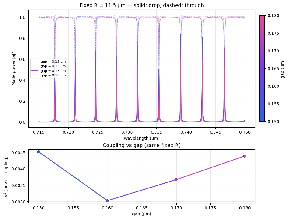
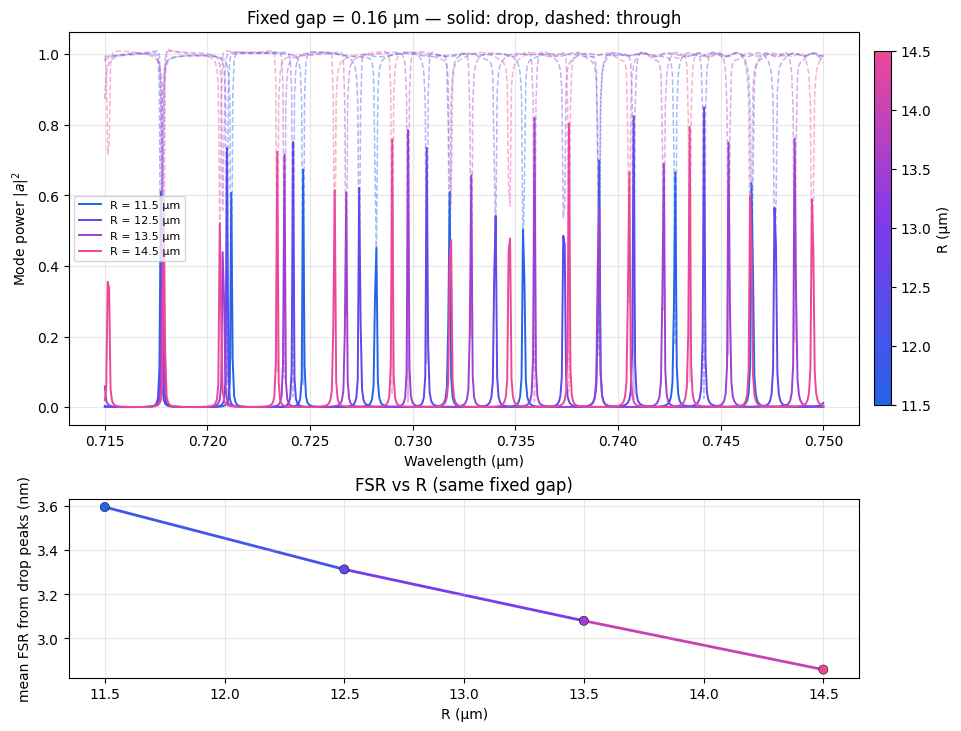
# Convert the sweep metric rows into radius-gap grids and plot compact heatmap summaries.
def _metric_grid(rows, key):
    Rs = np.array(sorted({float(r["R_um"]) for r in rows}))
    gs = np.array(sorted({float(r["gap_um"]) for r in rows}))
    Z = np.full((len(gs), len(Rs)), np.nan)
    for row in rows:
        i = np.where(gs == float(row["gap_um"]))[0][0]
        j = np.where(Rs == float(row["R_um"]))[0][0]
        Z[i, j] = float(row.get(key, np.nan))
    return Rs, gs, Z


if metric_rows:
    keys = [
        "Q_loaded",
        "Q_intrinsic",
        "mean_fsr_nm_peaks",
        "loss_dB_per_cm",
        "kappa2_power",
    ]
    titles = [r"$Q_L$", r"$Q_i$", "FSR from peaks (nm)", "Loss (dB/cm)", r"$\kappa^2$"]
    fig, axes = plt.subplots(2, 3, figsize=(11, 6.5), constrained_layout=True)
    axes = axes.ravel()
    for ax, key, title in zip(axes, keys, titles):
        Rs, gs, Z = _metric_grid(metric_rows, key)
        im = ax.imshow(
            Z,
            origin="lower",
            aspect="auto",
            extent=[Rs.min(), Rs.max(), gs.min(), gs.max()],
        )
        ax.set_xlabel("R (µm)")
        ax.set_ylabel("gap (µm)")
        ax.set_title(title)
        fig.colorbar(im, ax=ax, shrink=0.85)
    axes[-1].axis("off")
    fig.suptitle("2D EIA sweep metrics")
    plt.show()
else:
    print("No metric_rows available for heatmaps.")
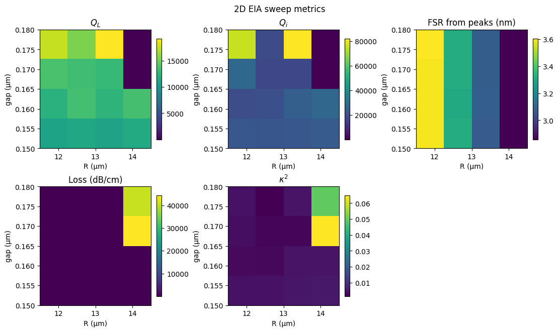
3.9 Full 3D Verification of Two Vernier Candidate Rings
The EIA sweep is useful for screening. The final candidate pair is verified with full 3D FDTD using the same ring builder. Here we simulate the two individual add-drop rings with radii 11.5 µm and 14.5 µm, then compare their resonance combs. Their slightly different FSRs produce the Vernier effect when the rings are later combined in a coupled architecture.
# Build full 3D simulations for the two shortlisted radii and inspect one layout.
sims_3d = {}
for R in VERNIER_RADII_UM:
    name = f"sin_mrr_R{R:g}_g{VERNIER_GAP_UM:g}"  # keep names compatible with parse_task_rg()
    sims_3d[name] = build_sin_ring_mrr_sim(
        R, VERNIER_GAP_UM, params=params
    )  # full 3D validation model

for name, sim in sims_3d.items():
    print(
        name,
        "| domain (µm):",
        tuple(round(x, 4) for x in sim.size),
        "| monitors:",
        [m.name for m in sim.monitors],
    )

first_name = next(iter(sims_3d))
fig, ax = plt.subplots(figsize=(7, 5.5))
sims_3d[first_name].plot(z=0, ax=ax)
ax.set_title(f"3D verification geometry: {first_name}")
ax.set_aspect("equal")
plt.tight_layout()
plt.show()
sin_mrr_R11.5_g0.16 | domain (µm): (24.5255, 25.8455, 1.2455) | monitors: ['drop', 'through', 'field']
sin_mrr_R14.5_g0.16 | domain (µm): (30.5255, 31.8455, 1.2455) | monitors: ['drop', 'through', 'field']
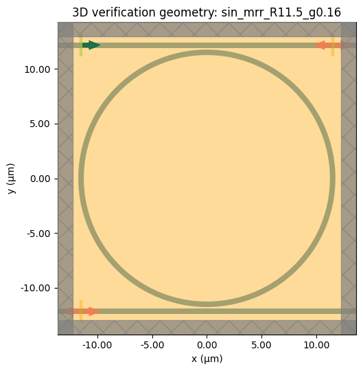
# Run the two-ring 3D verification batch only if its results are not already on disk.
VERNIER_3D_DIR = (
    Path("results") / "sin_vernier_rings_3d"
)  # output folder for 3D verification data
batch_3d = None  # populated only if a new run is needed
estimated_cost_3d = None  # populated by Batch.estimate_cost before running
batch_data_3d = None  # populated by the run, or loaded from disk in a later cell

if (VERNIER_3D_DIR / "batch.hdf5").exists():
    print("Loading existing 3D Vernier results from:", VERNIER_3D_DIR)
else:
    # Estimate the 3D verification cost before running. This does not time-step the
    # FDTD simulation, but it can create cloud task records.
    batch_3d = web.Batch(
        simulations=sims_3d, folder_name="sin_vernier_rings_715_750_3d"
    )
    estimated_cost_3d = batch_3d.estimate_cost(verbose=True)
    print(
        "Estimated maximum FlexCredits for the two-ring 3D verification batch:",
        estimated_cost_3d,
    )

    VERNIER_3D_DIR.mkdir(parents=True, exist_ok=True)
    batch_data_3d = batch_3d.run(path_dir=str(VERNIER_3D_DIR))
    print(batch_data_3d.task_ids)
16:53:57 -03 No Flexcredit cost for batch as all simulations were restored from
             local cache.
Estimated maximum FlexCredits for the two-ring 3D verification batch: 0.0
Found all simulations in cache.
{'sin_mrr_R11.5_g0.16': 'fdve-07808b1a-b298-497b-9614-4f9505ed9fd7', 'sin_mrr_R14.5_g0.16': 'fdve-b02b823d-ec00-4731-82ac-de7d3c06eaea'}
3.10 Load 3D Results, Compare Vernier Spectra, and Export Metrics
After running the 3D batch, the following cells load spectra, overlay the two candidate rings, and export the same through-notch metrics used for the EIA sweep. If a saved metrics CSV exists from a previous run, the final table can also be inspected directly.
# Load completed 3D results and overlay drop/through spectra for the Vernier candidates.
batch_data_3d = globals().get(
    "batch_data_3d", None
)  # reuse just-run 3D results if available
if batch_data_3d is None:
    batch_data_3d = load_batch_data(
        VERNIER_3D_DIR
    )  # otherwise load saved 3D batch data

spectra_3d = {}  # spectra keyed by radius/gap task name
if batch_data_3d is not None:
    for name, sim_data in batch_data_3d.items():
        wl_drop, T_drop = spectrum_mode_power(sim_data, "drop", "-")
        wl_through, T_through = spectrum_mode_power(sim_data, "through", "+")
        spectra_3d[name] = {
            "wl": wl_drop,
            "drop": T_drop,
            "through": np.interp(wl_drop, wl_through, T_through),
        }
    print(f"Loaded {len(spectra_3d)} 3D spectra.")
else:
    print(
        "No 3D BatchData loaded. Run the 3D batch or point VERNIER_3D_DIR to saved results."
    )

if spectra_3d:
    fig, axes = plt.subplots(1, 2, figsize=(11, 4.2), constrained_layout=True)
    for name, sp in spectra_3d.items():
        axes[0].plot(sp["wl"], sp["drop"], lw=1.3, label=f"{name}")
        axes[1].plot(sp["wl"], sp["through"], lw=1.3, label=f"{name}")
    axes[0].set_title("3D drop spectra: interleaved resonance combs")
    axes[1].set_title("3D through spectra: notch comparison")
    for ax in axes:
        ax.set_xlabel("Wavelength (µm)")
        ax.set_ylabel(r"Mode power $|a|^2$")
        ax.grid(True, alpha=0.3)
        ax.legend(fontsize=8)
    plt.show()
Loaded 2 3D spectra.
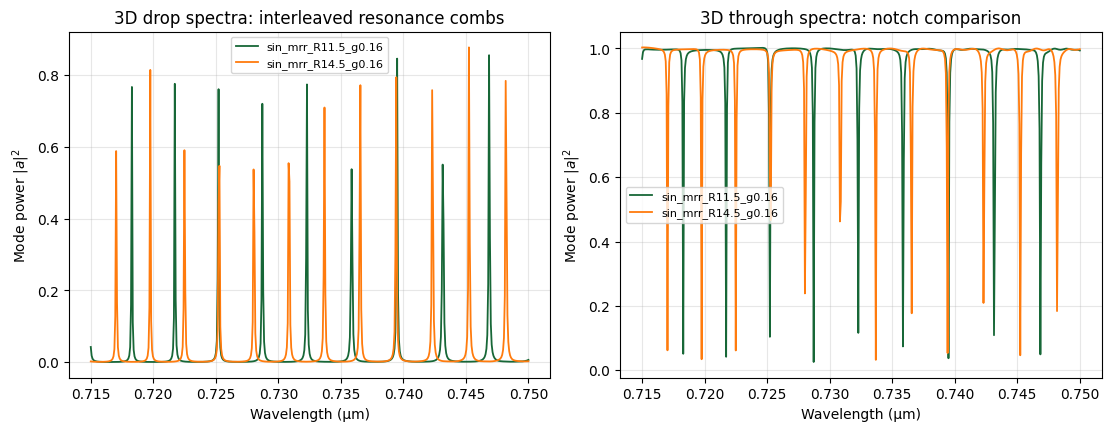
# Compute the same notch/FSR/Q/loss metrics for the 3D verification spectra.
metric_rows_3d = []  # one verification metric row per selected 3D ring
for name, sp in spectra_3d.items():
    R, g = parse_task_rg(name)
    metric_rows_3d.append(
        ring_metrics_row(
            name,
            R,
            g,
            sp["wl"],
            sp["drop"],
            sp["through"],
            lambda_fit_target_um=NOTCH_FIT_CENTER_UM,  # same target notch used for EIA comparison
            notch_half_width_um=NOTCH_HALF_WIDTH_UM,  # local 3D fitting window
            n_group_for_kappa2=N_GROUP_FOR_KAPPA2,  # group-index estimate for κ² / loss conversion
        )
    )

if metric_rows_3d:
    csv_path = VERNIER_3D_DIR / "community_vernier_ring_metrics.csv"
    csv_path.parent.mkdir(parents=True, exist_ok=True)
    with csv_path.open("w", newline="") as fp:
        writer = csv.DictWriter(
            fp, fieldnames=list(metric_rows_3d[0].keys()), extrasaction="ignore"
        )
        writer.writeheader()
        writer.writerows(metric_rows_3d)
    print(f"Wrote {len(metric_rows_3d)} 3D metric rows to {csv_path}")

    cols = [
        "task",
        "lambda0_um",
        "fwhm_nm",
        "Q_loaded",
        "Q_intrinsic",
        "Q_coupling",
        "mean_fsr_nm_peaks",
        "n_group_from_fsr",
        "kappa2_power",
        "loss_dB_per_cm",
        "coupling_regime",
    ]
    for row in metric_rows_3d:
        print("\n" + row["task"])
        for c in cols[1:]:
            print(f"  {c}: {row.get(c)}")
else:
    previous_csv = VERNIER_3D_DIR / "vernier_ring_metrics.csv"
    if previous_csv.is_file():
        print(f"No BatchData loaded, but previous metrics exist at {previous_csv}")
    else:
        print("No 3D metrics available yet.")
Wrote 2 3D metric rows to results/sin_vernier_rings_3d/community_vernier_ring_metrics.csv

sin_mrr_R11.5_g0.16
  lambda0_um: 0.7394927347627271
  fwhm_nm: 0.07204296118022299
  Q_loaded: 10264.607709735985
  Q_intrinsic: 20529.210609104277
  Q_coupling: 41058.44045968382
  mean_fsr_nm_peaks: 3.570000000000004
  n_group_from_fsr: 2.1199318429180414
  kappa2_power: 0.004878599970684205
  loss_dB_per_cm: 36.8478267757335
  coupling_regime: critical

sin_mrr_R14.5_g0.16
  lambda0_um: 0.7394209075871926
  fwhm_nm: 0.06963973336680075
  Q_loaded: 10617.80210576877
  Q_intrinsic: 21235.778844095883
  Q_coupling: 42470.859163702706
  mean_fsr_nm_peaks: 2.831818181818183
  n_group_from_fsr: 2.1191915631060025
  kappa2_power: 0.005947287845935092
  loss_dB_per_cm: 35.62526639398402
  coupling_regime: critical
4. SiN Grating Coupler
Linear Grating Coupler at 740 nm (Si₃N₄ on SiO₂)
Quasi-2D setup: finite thickness along y with PML (needed for FieldProjectionCartesianMonitor).
-
Excitation:
ModeSourceon the narrow ridge; optionalPolySlabtaper (narrow→wide toward the grating in xy). Usesim.plot(z≈0.11)to view xy outline. -
Monitors:
radiation_far(far field),mode_transmission(output waveguide — forward power in mode m is|a+|²in W vs the normalized mode source; callcoupling_efficiency_metrics(sim_data)), co-planarflux_output_waveguide(total +x flux for cross-check),field_xz_mid,flux_up_air. Defaults lean storage: Ey on the field monitor, spatialinterval_spacedownsampling, fewer transmitted modes (transmission_mode_num_modes), slightly smaller XY span and projection grid (far_field_nx).
Default stack (bottom → top): 2 µm Si, 5 µm SiO₂, 220 nm Si₃N₄, 5 µm SiO₂, then air. With a taper, narrow SiN width is core_width_um (input + taper start); grating slab/teeth match taper_input_width_um in y (same as wide taper side). Film-plane SiO₂ lateral strips exclude ±core_width_um/2 so oxide fills wedges beside the flaring rib.
Geometry parameters are illustrative—tune period_um, duty cycle, and etch for your stack.
Cloud runs use FlexCredit; only call web.run when you intend to solve remotely.
from __future__ import annotations

from typing import Any

import matplotlib.pyplot as plt
import numpy as np

import tidy3d as td
from tidy3d import material_library
Geometry and Simulation Builder
def _box(
    center: tuple[float, float, float],
    size: tuple[float, float, float],
    medium: td.Medium,
) -> td.Structure:
    return td.Structure(geometry=td.Box(center=center, size=size), medium=medium)


def make_linear_grating_coupler_simulation(
    wavelength_um: float = 0.74,
    period_um: float = 0.52,
    duty_cycle: float = 0.55,
    n_periods: int = 30,
    core_width_um: float = 0.5,
    core_nominal_um: float = 0.22,
    etch_um: float = 0.11,
    slab_thickness_um: float | None = None,
    straight_um: float = 2.8,
    taper_length_um: float = 0.0,
    taper_input_width_um: float = 2.0,
    box_um: float = 5.0,
    top_oxide_um: float = 5.0,
    bulk_si_thickness_um: float = 2.0,
    air_um: float = 2.5,
    domain_y_um: float | None = None,
    min_steps_per_wvl: int = 24,
    projection_height_um: float = 5.5,
    pml_layers: tuple[int, int, int] = (44, 40, 48),
    absorber_y: bool = True,
    absorber_layers_y: int | None = None,
    absorber_x: bool = True,
    absorber_layers_x: int | None = None,
    stable_z_pml: bool = True,
    stable_x_pml: bool = True,
    courant: float = 0.72,
    source_x_um: float | None = None,
    far_field_nx: int = 41,
    far_field_ny: int = 3,
    field_monitor_fields: tuple[str, ...] = ("Ey",),
    field_monitor_xy_fraction: tuple[float, float] = (0.35, 0.52),
    field_monitor_interval_space: tuple[int, int, int] = (2, 1, 2),
    field_projection_interval_space: tuple[int, int, int] = (2, 2, 1),
    transmission_mode_num_modes: int = 3,
) -> td.Simulation:
    slab_h = (
        slab_thickness_um
        if slab_thickness_um is not None
        else (core_nominal_um - etch_um)
    )
    slab_h = max(float(slab_h), 1e-3)

    si3n4_main = material_library["Si3N4"]["Luke2015Sellmeier"]
    sio2 = material_library["SiO2"]["Palik_Lossless"]
    si_bulk = material_library["cSi"]["Green2008"]

    freq0_hz = td.C_0 / wavelength_um
    fwidth_hz = freq0_hz * 0.15
    pulse = td.GaussianPulse(freq0=freq0_hz, fwidth=fwidth_hz)

    gr_len = period_um * n_periods
    x_g0 = -0.5 * gr_len
    x_g1 = 0.5 * gr_len
    strip_left = x_g0 - straight_um

    w_tap_in = float(taper_input_width_um)
    t_len = float(taper_length_um)
    use_taper = t_len > 1e-6 and w_tap_in > float(core_width_um) + 1e-6
    xt0 = max(strip_left, x_g0 - t_len) if use_taper else strip_left
    if use_taper and (x_g0 - xt0) < 1e-6:
        use_taper = False
    w_y_max = max(float(core_width_um), w_tap_in if use_taper else float(core_width_um))

    _cell_y_auto = max(2.05 * w_y_max, 2.1 * wavelength_um, w_y_max + wavelength_um)
    cell_y = domain_y_um if domain_y_um is not None else _cell_y_auto

    dev_half_x = abs(strip_left) + 2.65 * wavelength_um
    lx = 2.0 * dev_half_x

    z_intf = 0.0
    z_si_top = z_intf + core_nominal_um
    z_stack_top = z_si_top + float(top_oxide_um)
    oz_sz_z = float(box_um)
    z_bottom_oxide = z_intf - oz_sz_z
    z_bulk_bottom = z_bottom_oxide - float(bulk_si_thickness_um)
    zb_domain = z_bulk_bottom - 0.225 * wavelength_um
    z_domain_top = z_stack_top + air_um + wavelength_um * 0.62
    lz_domain = z_domain_top - zb_domain
    sim_center = (0.0, 0.0, zb_domain + 0.5 * lz_domain)

    z_padding_z = 0.55 * wavelength_um
    size_z = lz_domain + z_padding_z
    z_sim_min = sim_center[2] - 0.5 * size_z

    ridge_y_narrow = float(core_width_um)
    ridge_y_span = ridge_y_narrow
    ridge_grating_y = w_tap_in if use_taper else ridge_y_narrow

    structures: list[td.Structure] = []

    ox_y = max(lx * 0.085 + core_width_um * 24.0, 12.0 * wavelength_um)
    ox_x = lx * 3.28

    si_total_z = z_bottom_oxide - z_sim_min
    bulk_si = _box(
        center=(0.0, 0.0, z_sim_min + 0.5 * si_total_z),
        size=(ox_x, ox_y, si_total_z),
        medium=si_bulk,
    )
    structures.append(bulk_si)

    oxide_lower = _box(
        center=(0.0, 0.0, z_intf - 0.5 * oz_sz_z),
        size=(ox_x, ox_y, oz_sz_z),
        medium=sio2,
    )
    structures.append(oxide_lower)

    # Lateral SiO2 in film plane: exclude ±half(core_width) only—fills wedges beside widening taper.
    ox_half = 0.5 * ox_x
    oy_half = 0.5 * ox_y
    ridge_half_clad = 0.5 * float(core_width_um)
    side_y_sz = oy_half - ridge_half_clad
    if side_y_sz > 1e-6:
        z_core_mid = z_intf + 0.5 * core_nominal_um
        structures.append(
            _box(
                center=(0.0, -0.5 * (oy_half + ridge_half_clad), z_core_mid),
                size=(ox_x, side_y_sz, core_nominal_um),
                medium=sio2,
            )
        )
        structures.append(
            _box(
                center=(0.0, 0.5 * (oy_half + ridge_half_clad), z_core_mid),
                size=(ox_x, side_y_sz, core_nominal_um),
                medium=sio2,
            )
        )

    # Uniform Si3N4 film on the input side (before the ridge/grating footprint in +x).
    # Use ridge_y_narrow in y — not w_y_max — so width matches the narrow rib and taper start at strip_left.
    if strip_left > -ox_half + 1e-6:
        lx_in = strip_left + ox_half
        structures.append(
            _box(
                center=(strip_left - 0.5 * lx_in, 0.0, z_intf + 0.5 * core_nominal_um),
                size=(lx_in, ridge_y_narrow, core_nominal_um),
                medium=si3n4_main,
            )
        )

    straight_top = core_nominal_um - slab_h
    if use_taper:
        w_in = w_tap_in
        half_in = 0.5 * w_in
        half_gr = 0.5 * ridge_y_narrow
        if xt0 > strip_left + 1e-6:
            x_u0, x_u1 = strip_left, xt0
            len_u = x_u1 - x_u0
            structures.append(
                _box(
                    center=(x_u0 + 0.5 * len_u, 0.0, z_intf + 0.5 * slab_h),
                    size=(len_u, ridge_y_span, slab_h),
                    medium=si3n4_main,
                )
            )
            if straight_top > 1e-4:
                structures.append(
                    _box(
                        center=(
                            x_u0 + 0.5 * len_u,
                            0.0,
                            z_intf + slab_h + 0.5 * straight_top,
                        ),
                        size=(len_u, ridge_y_span, straight_top),
                        medium=si3n4_main,
                    )
                )
        taper_geo = td.PolySlab(
            vertices=[
                (xt0, -half_gr),
                (x_g0, -half_in),
                (x_g0, half_in),
                (xt0, half_gr),
            ],
            axis=2,
            slab_bounds=(z_intf, z_si_top),
        )
        structures.append(td.Structure(geometry=taper_geo, medium=si3n4_main))
        slab_len_gr = x_g1 - x_g0
        structures.append(
            _box(
                center=(x_g0 + 0.5 * slab_len_gr, 0.0, z_intf + 0.5 * slab_h),
                size=(slab_len_gr, ridge_grating_y, slab_h),
                medium=si3n4_main,
            )
        )
    else:
        slab_len = x_g1 - strip_left
        slab_center_x = strip_left + 0.5 * slab_len
        structures.append(
            _box(
                center=(slab_center_x, 0.0, z_intf + 0.5 * slab_h),
                size=(slab_len, ridge_y_span, slab_h),
                medium=si3n4_main,
            )
        )
        if straight_top > 1e-4:
            structures.append(
                _box(
                    center=(
                        (strip_left + x_g0) * 0.5,
                        0.0,
                        z_intf + slab_h + 0.5 * straight_top,
                    ),
                    size=(x_g0 - strip_left, ridge_y_span, straight_top),
                    medium=si3n4_main,
                )
            )

    if x_g1 < ox_half - 1e-6:
        rx_pad = ox_half - x_g1
        structures.append(
            _box(
                center=(x_g1 + 0.5 * rx_pad, 0.0, z_intf + 0.5 * core_nominal_um),
                size=(rx_pad, ox_y, core_nominal_um),
                medium=sio2,
            )
        )

    tooth_w = duty_cycle * period_um
    top_h = core_nominal_um - slab_h
    if top_h > 1e-4:
        gr_len_x = x_g1 - x_g0
        structures.append(
            _box(
                center=(0.5 * (x_g0 + x_g1), 0.0, z_intf + slab_h + 0.5 * top_h),
                size=(gr_len_x, ridge_grating_y, top_h),
                medium=sio2,
            )
        )
    for k in range(n_periods):
        xc = x_g0 + (k + 0.5 * duty_cycle) * period_um
        if top_h <= 1e-4:
            break
        structures.append(
            _box(
                center=(xc, 0.0, z_intf + slab_h + 0.5 * top_h),
                size=(tooth_w * 0.996, ridge_grating_y, top_h),
                medium=si3n4_main,
            )
        )

    top_ox_t = float(top_oxide_um)
    oxide_top = _box(
        center=(0.0, 0.0, z_si_top + 0.5 * top_ox_t),
        size=(ox_x, ox_y, top_ox_t),
        medium=sio2,
    )
    structures.append(oxide_top)

    src_x = 0.5 * (strip_left + x_g0) if source_x_um is None else float(source_x_um)
    src_z = z_intf + min(0.48 * core_nominal_um, 0.55 * z_si_top)
    mode_h = min(2.6 * wavelength_um, air_um * 0.78 + core_nominal_um)
    mode_sz_y = max(6.0 * w_y_max, cell_y, 0.8 * wavelength_um)
    ms = td.ModeSource(
        center=(src_x, 0.0, src_z),
        size=(0.0, mode_sz_y, mode_h),
        source_time=pulse,
        direction="+",
        mode_spec=td.ModeSpec(num_modes=8, target_neff=1.45),
        mode_index=0,
        num_freqs=3,
    )

    collection_span = min(lx * 0.41, gr_len + 10.0 * wavelength_um)
    z_collect = sim_center[2] + 0.5 * lz_domain - 0.38 * wavelength_um
    z_origin = z_si_top + 0.35 * top_ox_t
    proj_y = max(4.0 * w_y_max, 0.25 * wavelength_um)
    _ff_nx = max(3, int(far_field_nx))
    _ff_ny = max(1, int(far_field_ny))
    _fpi_x, _fpi_y, _fpi_z = (
        max(1, int(field_projection_interval_space[i])) for i in range(3)
    )
    nf_monitor = td.FieldProjectionCartesianMonitor(
        center=(gr_len * 0.048, 0.0, z_collect - wavelength_um),
        size=(collection_span, proj_y, 0.0),
        freqs=[freq0_hz],
        name="radiation_far",
        custom_origin=(0.0, 0.0, z_origin),
        x=np.linspace(-collection_span / 2.06, collection_span / 2.06, _ff_nx).tolist(),
        y=np.linspace(-0.12 * cell_y, 0.12 * cell_y, _ff_ny).tolist(),
        proj_axis=2,
        proj_distance=projection_height_um,
        far_field_approx=False,
        interval_space=(_fpi_x, _fpi_y, _fpi_z),
    )

    field_y = max(0.35 * w_y_max, 0.02 * wavelength_um)
    _fx, _fz = float(field_monitor_xy_fraction[0]), float(field_monitor_xy_fraction[1])
    _fmx, _fmy, _fmz = (max(1, int(field_monitor_interval_space[i])) for i in range(3))
    fz = td.FieldMonitor(
        center=(
            src_x + 5.08 * wavelength_um + gr_len * 0.52,
            0.0,
            z_intf + wavelength_um,
        ),
        size=(lx * _fx, field_y, lz_domain * _fz),
        freqs=[freq0_hz],
        name="field_xz_mid",
        fields=tuple(field_monitor_fields),
        interval_space=(_fmx, _fmy, _fmz),
    )

    flux_z = sim_center[2] + 0.5 * lz_domain - 0.35 * wavelength_um
    flux_up = td.FluxMonitor(
        center=(gr_len * 0.02, 0.0, flux_z),
        size=(lx * 0.42, field_y, 0.0),
        freqs=[freq0_hz],
        name="flux_up_air",
        normal_dir="+",
    )

    trans_x = x_g1 + max(2.0 * wavelength_um, 0.35 * straight_um)
    _n_tm = max(1, int(transmission_mode_num_modes))
    mode_trans = td.ModeMonitor(
        center=(trans_x, 0.0, src_z),
        size=(0.0, mode_sz_y, mode_h),
        freqs=[freq0_hz],
        name="mode_transmission",
        mode_spec=td.ModeSpec(num_modes=_n_tm, target_neff=1.45),
        colocate=False,
    )
    flux_output = td.FluxMonitor(
        center=(trans_x, 0.0, src_z),
        size=(0.0, mode_sz_y, mode_h),
        freqs=[freq0_hz],
        name="flux_output_waveguide",
        normal_dir="+",
    )

    nx_pml, ny_pml, nz_pml = pml_layers
    ny_abs = absorber_layers_y if absorber_layers_y is not None else max(ny_pml + 8, 56)
    nx_abs = absorber_layers_x if absorber_layers_x is not None else max(nx_pml + 8, 56)
    if absorber_x:
        x_bnd = td.Boundary.absorber(num_layers=nx_abs)
    elif stable_x_pml:
        x_bnd = td.Boundary.stable_pml(num_layers=nx_pml)
    else:
        x_bnd = td.Boundary.pml(num_layers=nx_pml)
    z_bnd = (
        td.Boundary.stable_pml(num_layers=nz_pml)
        if stable_z_pml
        else td.Boundary.pml(num_layers=nz_pml)
    )
    if absorber_y:
        boundary_spec = td.BoundarySpec(
            x=x_bnd,
            y=td.Boundary.absorber(num_layers=ny_abs),
            z=z_bnd,
        )
    else:
        boundary_spec = td.BoundarySpec(
            x=x_bnd,
            y=td.Boundary.pml(num_layers=ny_pml),
            z=z_bnd,
        )

    grid = td.GridSpec(
        grid_x=td.AutoGrid(min_steps_per_wvl=min_steps_per_wvl),
        grid_y=td.AutoGrid(min_steps_per_wvl=min_steps_per_wvl),
        grid_z=td.AutoGrid(min_steps_per_wvl=min_steps_per_wvl),
        wavelength=wavelength_um,
    )

    run_time = td.RunTimeSpec(quality_factor=6.4, source_factor=3.2)

    sim_kw: dict[str, Any] = dict(
        size=(lx + 1.75 * wavelength_um, cell_y, size_z),
        center=sim_center,
        medium=td.Medium(permittivity=1.0),
        symmetry=(0, 0, 0),
        structures=tuple(structures),
        boundary_spec=boundary_spec,
        grid_spec=grid,
        sources=(ms,),
        monitors=(fz, flux_up, nf_monitor, mode_trans, flux_output),
        run_time=run_time,
        subpixel=True,
        courant=float(courant),
    )
    return td.Simulation(**sim_kw)
Post-Processing Helpers (after web.run)
-
coupling_efficiency_metrics(sim_data)— forward/backward modal powers atmode_transmissionand total +x flux onflux_output_waveguide(cross-check vs sum of modes).
def postprocess_cartesian_projection(sim_data: td.SimulationData) -> dict[str, Any]:
    """Lightweight metrics from the Cartesian far-field projection monitor."""
    pdata = sim_data["radiation_far"]
    out: dict[str, Any] = {"monitor": pdata}
    for comp in ("Er", "Etheta", "Ephi"):
        arr = getattr(pdata, comp, None)
        if arr is None:
            continue
        v = np.asarray(arr.values, dtype=complex)
        out[f"rms_{comp}"] = float(np.sqrt(np.mean(np.abs(v) ** 2)))
    return out


def coupling_efficiency_metrics(sim_data: td.SimulationData) -> dict[str, Any]:
    """Power coupled into waveguide modes at ``mode_transmission`` (see Fluxcompute FAQ).

    With a ``ModeSource``, monitor fields are normalized to the source spectrum; at the
    central frequency the injected power is ~1 W. Forward modal power is ``|a+|²`` in watts.

    References:
    https://docs.flexcompute.com/projects/tidy3d/en/latest/faq/docs/faq/how-do-i-get-the-coupling-efficiency-of-a-specific-waveguide-mode.html
    """
    md = sim_data["mode_transmission"]
    amps_f = md.amps.sel(direction="+")
    amps_b = md.amps.sel(direction="-")
    p0_f = md.amps.sel(mode_index=0, direction="+")
    p0_b = md.amps.sel(mode_index=0, direction="-")
    out: dict[str, Any] = {
        "power_forward_mode0_W": float(np.sum(np.abs(p0_f.values) ** 2)),
        "power_forward_all_tracked_modes_W": float(np.sum(np.abs(amps_f.values) ** 2)),
        "power_backward_mode0_W": float(np.sum(np.abs(p0_b.values) ** 2)),
        "power_backward_all_tracked_modes_W": float(np.sum(np.abs(amps_b.values) ** 2)),
    }
    try:
        fx = sim_data["flux_output_waveguide"].flux
        out["flux_output_waveguide_W"] = float(np.squeeze(fx.values))
    except KeyError:
        pass
    return out
Build, Inspect, and Run
The taper widens the rib in xy toward +x (half-width grows toward taper_input_width_um at x_g0). A sim.plot(y=0) xz cut still tends to look like a rectangle at the centerline; use sim.plot(z≈0.11 µm) for xy geometry.
Run sim.plot(y=0) for xz, sim.plot(z≈0.11) for xy (taper outline), and sim.plot(z=0.26) for xy in upper SiO₂. Use sim.validate() for a structural check.
The grating coupler is run automatically in the next cell; if a saved result already exists it is loaded instead of resubmitting.
sim = make_linear_grating_coupler_simulation(
    taper_length_um=2.0,
    taper_input_width_um=1.8,
    source_x_um=-10.5,
)

print("size (µm):", [round(s, 5) for s in sim.size])
print("monitors:", [m.name for m in sim.monitors])
print("run_time (s):", f"{sim._run_time:.4e}")

_, ax = plt.subplots(figsize=(8, 4))
_ = sim.plot(y=0, ax=ax)
_ = ax.set_title("Cross-section at y = 0 (xz)")
plt.tight_layout()
plt.show()
size (µm): [26.417, 3.69, 15.7523]
monitors: ['field_xz_mid', 'flux_up_air', 'radiation_far', 'mode_transmission', 'flux_output_waveguide']
run_time (s): 1.2334e-12
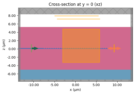
# Run the grating coupler (or load it if already saved) so the result summary below has data.
GRATING_DATA_PATH = DATA_DIR / "grating_coupler_sim_data.hdf5"
if GRATING_DATA_PATH.exists():
    sim_data = td.SimulationData.from_file(str(GRATING_DATA_PATH))
    print("Loaded grating-coupler data from:", GRATING_DATA_PATH)
else:
    sim_data = web.run(
        sim,
        task_name="sin_grating_coupler_740nm",
        path=str(GRATING_DATA_PATH),
        verbose=True,
    )
16:53:58 -03 Loading simulation from local cache. View cached task using web UI
             at
             'https://tidy3d.simulation.cloud/workbench?taskId=fdve-dfd1b298-9f5
             f-4d3d-b6df-74da3f0c99fa'.
Extra Diagnostic: Geometry and Monitor Summary
This cell summarizes the simulation size, number of structures, sources, and monitors.
It is useful for checking whether the grating coupler simulation contains the expected waveguide, grating region, source, field monitor, flux monitor, and far-field monitor before running the simulation.
print("=== Geometry and monitor summary ===")

print("Simulation size [x, y, z] in µm:")
print([round(v, 4) for v in sim.size])

print("\nNumber of structures:")
print(len(sim.structures))

print("\nSources:")
for src in sim.sources:
    print(f"- {src.name}: center={src.center}, size={src.size}")

print("\nMonitors:")
for mon in sim.monitors:
    print(f"- {mon.name}: center={mon.center}, size={mon.size}")
=== Geometry and monitor summary ===
Simulation size [x, y, z] in µm:
[26.417, 3.69, 15.7523]

Number of structures:
42

Sources:
- None: center=(-10.5, 0.0, 0.1056), size=(0.0, 10.8, 1.924)

Monitors:
- field_xz_mid: center=(1.3712000000000018, 0.0, 0.74), size=(8.7927, 0.63, 7.979556)
- flux_up_air: center=(0.31200000000000006, 0.0, 7.919799999999999), size=(10.551240000000002, 0.63, 0.0)
- radiation_far: center=(0.7488000000000001, 0.0, 7.157599999999999), size=(10.30002, 7.2, 0.0)
- mode_transmission: center=(9.280000000000001, 0.0, 0.1056), size=(0.0, 10.8, 1.924)
- flux_output_waveguide: center=(9.280000000000001, 0.0, 0.1056), size=(0.0, 10.8, 1.924)
Cross-Section in the xy Plane (Taper Widens Toward Grating)
Use sim.plot(z=h) with h inside the 220 nm Si₃N₄ film (e.g. 0.11 µm, mid film with z_intf=0). Film-plane SiO₂ fills y outside ±core_width_um/2 (not only outside the taper width), so wedges beside the widening rib are oxide—not air.
With z_si_top ≈ 0.22 µm, z = 0.26 µm lies in the upper SiO₂ cladding (wide oxide above the rib). See Tidy3D Simulation.plot.
z_mid_film_um = 0.0  # inside SiN film — xy taper outline
z_upper_oxide_um = 0.22  # in top SiO2 cladding

_, ax_mid = plt.subplots(figsize=(6, 5))
_ = sim.plot(z=z_mid_film_um, ax=ax_mid)
_ = ax_mid.set_title(f"xy at z = {z_mid_film_um} µm (mid nitride — taper nar→wide)")
plt.tight_layout()
plt.show()

_, ax_up = plt.subplots(figsize=(6, 5))
_ = sim.plot(z=z_upper_oxide_um, ax=ax_up)
_ = ax_up.set_title(f"xy at z = {z_upper_oxide_um} µm (upper SiO₂)")
plt.tight_layout()
plt.show()
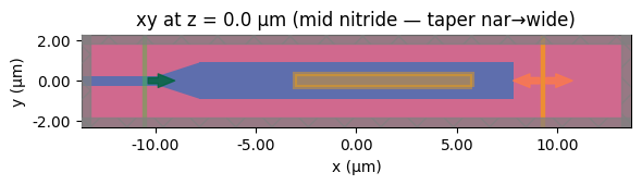
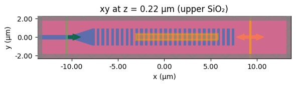
Extra Diagnostic: Grating Coupler Result Summary
This cell summarizes the main physical results of the SiN grating coupler simulation.
It reports the coupling-efficiency-related metrics, upward radiated flux, and far-field strength.
These quantities help evaluate whether the input waveguide mode is efficiently radiated upward by the grating coupler.
print("=== Grating coupler result summary ===")

# Coupling-efficiency-related metrics
try:
    ce_metrics = coupling_efficiency_metrics(sim_data)

    print("\nCoupling efficiency metrics:")
    for key, value in ce_metrics.items():
        print(f"{key}: {value:.6g}")

except Exception as e:
    print("\nCould not calculate coupling efficiency metrics:")
    print(e)


# Upward radiation flux
try:
    flux_up = sim_data["flux_up_air"].flux
    flux_up_value = float(np.squeeze(flux_up.values))

    print("\nUpward radiation flux:")
    print(f"{flux_up_value:.6g}")

except Exception as e:
    print("\nCould not read upward radiation flux:")
    print(e)


# Far-field strength summary
try:
    ff_metrics = postprocess_cartesian_projection(sim_data)

    print("\nFar-field RMS strength:")
    for key, value in ff_metrics.items():
        if key.startswith("rms"):
            print(f"{key}: {value:.6g}")

except Exception as e:
    print("\nCould not calculate far-field metrics:")
    print(e)
=== Grating coupler result summary ===

Coupling efficiency metrics:
power_forward_mode0_W: 5.35562e-07
power_forward_all_tracked_modes_W: 0.125941
power_backward_mode0_W: 2.79422e-09
power_backward_all_tracked_modes_W: 0.00015726
flux_output_waveguide_W: 0.366555

Upward radiation flux:
0.0011966

Far-field RMS strength:
rms_Er: 0.271187
rms_Etheta: 0.441152
rms_Ephi: 0.331177