





# standard python imports
import gdstk
import matplotlib as mpl
import matplotlib.pyplot as plt
import numpy as np
import scipy

# tidy3D import
import tidy3d as td
import tidy3d.web as web
TIDY3D
LEARNING CENTER
Example Library

Bistability in photonic crystal microcavities
Introduction
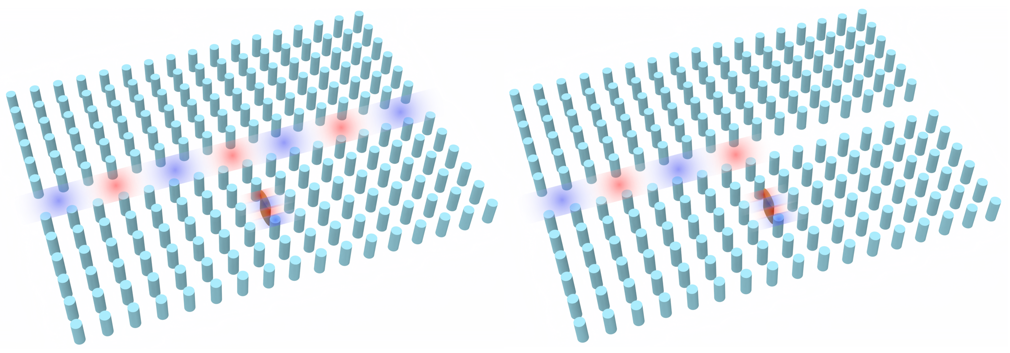
Here we take advantage of Tidy3D’s nonlinear capability to demonstrate optical bistability. We base this example on the paper from Yanik et al. titled High-contrast all-optical bistable switching in photonic crystal microcavities. In this paper, a photonic crystal waveguide coupled with a point-defect cavity with Kerr nonlinearity achieves high-contrast transmission between two stable states.
For more simulation examples, please visit our examples page. If you are new to the finite-difference time-domain (FDTD) method, we highly recommend going through our FDTD101 tutorials. FDTD simulations can diverge due to various reasons. If you run into any simulation divergence issues, please follow the steps outlined in our troubleshooting guide to resolve it.
Setup
We first import the packages we’ll need.
The waveguide-cavity system we examine is given by a square lattice (with lattice constant a) of high dielectric rods (\(n\) = 3.5) of radius \(.2a\). The waveguide is given by removing a row of these rods, and the cavity is given by a point defect in the crystal - instead of a rod, the defect is an ellipse with major and minor axes of \(a\) and \(2a\), respectively. Here we will set \(a\) = 1.
To build this in Tidy3D, we take advantage of the “square_cylinder_array” method in the common photonic crystal structures page in the Tidy3D learning center.
Since we are dealing with a photonic crystal with discrete translational symmetry, we can get spurious reflections if we simply use a PML boundary condition. Thus, instead we use the custom absorbing condition given in Mekis et al.’s Absorbing boundary conditions for FDTD simulations of photonic crystal waveguides. This is a \(k\)-matched distributed Bragg reflector waveguide consisting of a periodic array of alternating periodic slabs, with the waveguide given by a single line defect of a single slab with larger thickness. Since this waveguide has continuous translational symmetry, we can now feed it into a standard PML boundary. For simplicity, in defining the parameters for this waveguide, we use the parameters given in Mekis et al.
def square_cylinder_array(
    x0,
    y0,
    z0,
    R,
    hole_spacing_x,
    hole_spacing_y,
    n_x,
    n_y,
    height,
    medium,
    reference_plane="bottom",
    sidewall_angle=0,
    axis=2,
):
    # parameters
    # ------------------------------------------------------------
    # x0: x coordinate of center of the array (um)
    # y0: y coordinate of center of the array (um)
    # z0: z coordinate of center of the array (um)
    # R: radius of the circular holes (um)
    # hole_spacing_x: distance between centers of holes in x direction (um)
    # hole_spacing_y: distance between centers of holes in y direction (um)
    # n_x: number of cylinders in x direction
    # n_y: number of cylinders in y direction
    # height: height of array
    # medium: medium of the cylinders
    # reference_plane
    # sidewall_angle: angle slant of cylinders
    # axis

    cylinder_group = []

    start_x, start_y = x0 + hole_spacing_x * (1 - n_x) / 2, y0 + hole_spacing_y * (1 - n_y) / 2
    for i in range(0, n_x):
        for j in range(0, n_y):
            c = td.Cylinder(
                axis=axis,
                sidewall_angle=sidewall_angle,
                reference_plane=reference_plane,
                radius=R,
                center=(start_x + i * hole_spacing_x, start_y + j * hole_spacing_y, z0),
                length=height,
            )
            cylinder_group.append(c)
    structure = td.Structure(geometry=td.GeometryGroup(geometries=cylinder_group), medium=medium)
    return structure


def DBR(
    x0,
    y0,
    z0,
    length,
    thickness,
    spacing,
    num_layers,
    medium,
    direction="+",
):
    # parameters
    # ------------------------------------------------------------
    # x0: x coordinate of center of the array (um)
    # y0: y coordinate of center of the array (um)
    # z0: z coordinate of center of the array (um)
    # length: Length of slabs
    # thickness: thickness of slabs (um)
    # spacing: space between each slab (um)
    # num_layers: number of slabs
    # medium: medium of the slabs
    # direction: does it extend right or left from the center?

    slab_group = []
    orientation = 1
    if direction != "+":
        orientation = -1
    start_x, start_y = x0 + orientation * length / 2, y0 - num_layers / 2 * a
    for i in range(0, num_layers + 1):
        if i != num_layers // 2:
            s = td.Box(center=(start_x, start_y + i * a, 0), size=(length, thickness, td.inf))
            slab_group.append(s)
    structure = td.Structure(geometry=td.GeometryGroup(geometries=slab_group), medium=medium)
    return structure
Define Structure
We now carve out our waveguide and introduce or ellipse point defect. While the end goal of this notebook is to take advantage of the ellipse’s nonlinearity, we must first find the resonant frequency of the cavity when it behaves linearly - thus we set the material as a linear material for now.
We also want to compute \(\kappa\), a nonlinear feedback parameter crucial to our simulations - more on this later.
n_rods = 3.5
rod = td.Medium(permittivity=n_rods**2)
n_air = 1
air = td.Medium(permittivity=n_air)

# Kerr coefficient
n2 = 1.5e-17  # m^2/W, from paper
n2 *= 1e12  # convert to um^2/W

a = 1
radius = 0.2 * a
block_rows = 21
block_cols = 17

# ######################## SIMPLE CRYSTAL ##########################
block = square_cylinder_array(
    0, 0, -a, radius, a, a, block_cols, block_rows, td.inf, rod, reference_plane="middle"
)
# ######################## WAVEGUIDE WITHOUT CAVITY ##########################
waveguide = td.Structure(
    geometry=td.Box(
        center=[0, 0, 0],
        size=[td.inf, a, td.inf],
    ),
    medium=air,
    name="waveguide",
)
# ########################## WAVEGUIDE WITH CAVITY ###########################
cavity_air = td.Structure(
    geometry=td.Box(
        center=[0, -3 * a, 0],
        size=[a, a, td.inf],
    ),
    medium=air,
    name="cavity air",
)
air_block = td.Structure(
    geometry=td.Box(
        center=[-22 * a, 0, 0],
        size=[30 * a - a / 2, td.inf, td.inf],
    ),
    medium=air,
    name="air block",
)

# ################## DISTRIBUTED BRAGG REFLECTOR BOUNDARY ###################
thickness = 0.25 * a
n_DBR = 10.2
dbr_med = td.Medium(permittivity=n_DBR**2)
dbr_boundary = DBR(block_cols * a / 2, 0, 0, 20, thickness, a, block_rows - 1, dbr_med)

# ################################# CAVITY ##################################
major = a
minor = 0.2 * a
cavity_gdstk = gdstk.ellipse((0, -3 * a), (minor / 2, major / 2))
cavity_cell = gdstk.Cell("Ellipse")
cavity_cell.add(cavity_gdstk)
cavity = td.PolySlab.from_gds(
    cavity_cell,
    gds_layer=0,
    gds_dtype=0,
    axis=2,
    slab_bounds=(-td.inf, td.inf),
    reference_plane="bottom",
)[0]

cavity_structure = td.Structure(
    geometry=cavity,
    medium=rod,
)
freqs = np.linspace(1.08e14, 1.1e14, 1000)
freq0 = freqs[len(freqs) // 2]
fwidth = freqs[-1] - freqs[0]
run_time = 10000 / freq0
# simulation parameters
x_span = 27 * a
y_span = 17 * a
min_steps_per_wvl = 30
gridSpecUniform = td.GridSpec.uniform(dl=a / 24)
pulse = td.GaussianPulse(freq0=freq0, fwidth=fwidth)
source_distance = 9
gaussianBeam = td.GaussianBeam(
center=[-source_distance * a, 0, 0],
size=[0, td.inf, td.inf],
source_time=pulse,
direction="+",
pol_angle=np.pi / 2,
waist_radius=2.0 * a,
)Things to Compute in the Linear Case
We wish to compute the resonant frequency \(\omega_{res}\) and the characteristic power of the cavity, given by
\(P_0=1/[\kappa Q^2 n_2 /c]\)
where \(Q\) is the cavity quality factor, \(n_2\) is the Kerr coefficient we’ll use, and \(\kappa\) is a nonlinear feedback parameter, a measure of the efficiency of the feedback system. We then use this to compute the cavity decay rate \(\gamma=\omega_{res}/(2Q)\).
To compute \(\omega_{res}\) and \(Q\), we use Tidy3D’s resonance finder.
In computing \(\kappa\), we use the definition given by Soljacic et al. in Optimal bistable switching in nonlinear photonic crystals:
\(\kappa=(\frac{c}{\omega_{res}})^2\frac{\int d^2r[|E(r)\cdot E(r)|^2 + 2|E(r)\cdot E^*(r)|^2]n^2(r)n_2(r)}{[\int d^2r|E(r)|^2n^2(r)]^2n_2}\)
Define Monitors and Simulation
We now input our monitors - a field monitor and permittivity monitor over the extent of the cavity’s mode to compute \(\kappa\) (field_monitor_cavity and permittivity_monitor_cavity), a field time monitor to compute our resonant frequency and cavity quality factor (field_time_monitor_wg), and a flux monitor at the end of the waveguide to find transmission vs frequency (flux_monitor).
cavity_monitor_size = 7
field_monitor_cavity = td.FieldTimeMonitor(
    fields=["Ez"],
    center=[0, -3 * a, 0],
    size=[cavity_monitor_size * a, cavity_monitor_size * a, 0],
    start=run_time * 8 / 10,
    stop=run_time * 8 / 10,
    name="field cavity",
)
permittivity_monitor_cavity = td.PermittivityMonitor(
    center=[0, -3 * a, 0],
    size=[cavity_monitor_size * a, cavity_monitor_size * a, 0],
    freqs=freqs[0],
    name="permittivity cavity",
)

flux_distance = 4.5

field_time_monitor_wg = td.FieldTimeMonitor(
    fields=["Ez"],
    center=[flux_distance * a, 0, 0],
    size=(0, 0, 0),
    start=run_time
    * 8
    / 10,  # time to start monitoring after source has decayed, units of 1/frequency bandwidth
    name="field time wg",
)
flux_monitor = td.FluxMonitor(
    center=[flux_distance * a, 0, 0],
    size=[0, td.inf, td.inf],
    freqs=freqs,
    normal_dir="+",
    name="flux",
)

x_boundary = td.Boundary(minus=td.PML(num_layers=80), plus=td.PML(num_layers=80))

sim_linear = td.Simulation(
    center=(0, -a, 0),
    size=[x_span, y_span, 0],
    medium=air,
    grid_spec=gridSpecUniform,
    structures=[block, waveguide, cavity_air, cavity_structure, dbr_boundary, air_block],
    sources=[gaussianBeam],
    monitors=[
        field_monitor_cavity,
        permittivity_monitor_cavity,
        field_time_monitor_wg,
        flux_monitor,
    ],
    run_time=run_time,
    boundary_spec=td.BoundarySpec(x=x_boundary, y=td.Boundary.periodic(), z=td.Boundary.periodic()),
    shutoff=False,
)
Visualize Simulation
sim_linear.plot(z=0)
plt.show()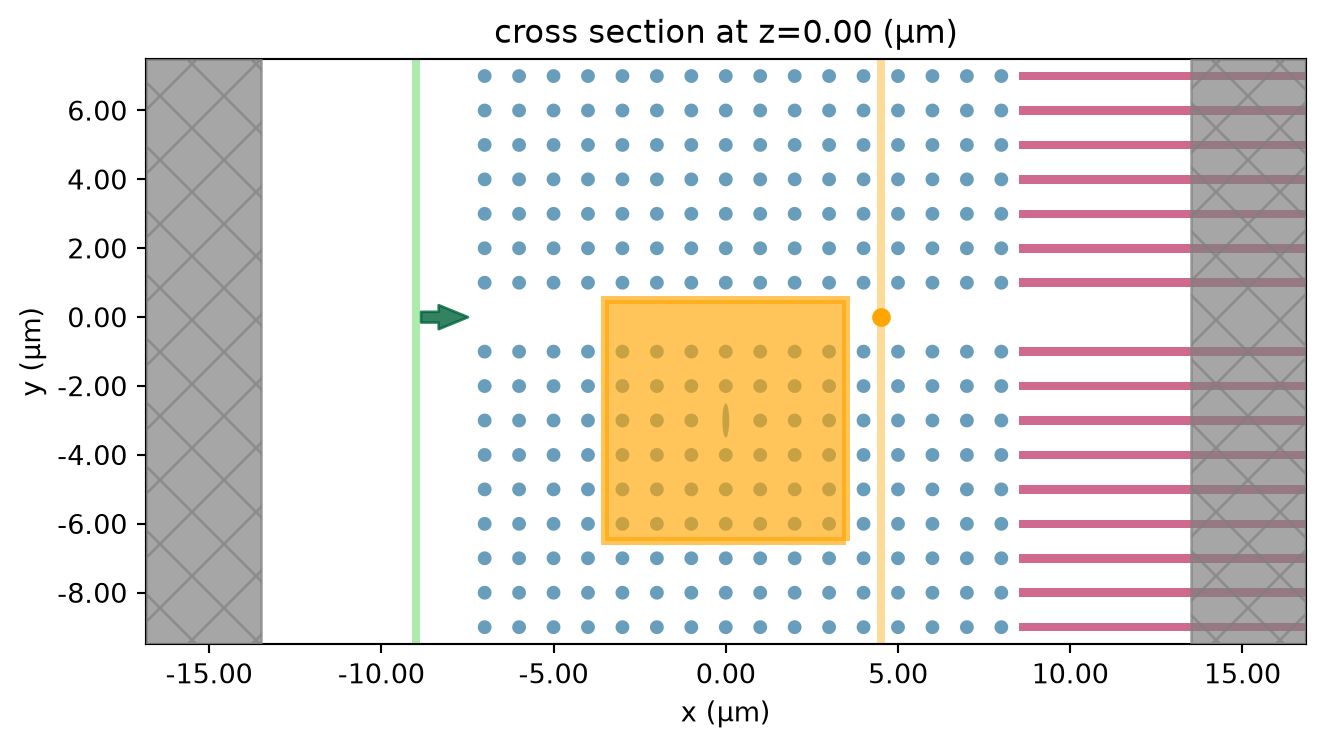
Run Simulation
sim_linear_data = web.run(sim_linear, task_name="bistable_pc_cavity")03:10:26 UTC Created task 'bistable_pc_cavity' with resource_id 'fdve-d808890e-ad62-485f-b6ad-bf229be9543e' and task_type 'FDTD'.
             View task using web UI at
             'https://tidy3d.simulation.cloud/workbench?taskId=fdve-d808890e-ad6
             2-485f-b6ad-bf229be9543e'.
Task folder: 'default'.
03:10:28 UTC Estimated FlexCredit cost: 0.097. This assumes the FDTD solver runs
             for the full simulation time; if early shutoff is reached, the
             billed cost can be lower. Use 'web.real_cost(task_id)' to get the
             billed FlexCredit cost after a simulation run.
03:10:29 UTC status = success
03:10:31 UTC Loading results from simulation_data.hdf5
Calculate Linear Resonance
We plot the flux through the waveguide vs frequency to verify that the the transmission vanishes on cavity resonance.
flx_cavity = sim_linear_data["flux"].flux
plt.plot(freqs, flx_cavity, label="Output Flux")
plt.xlabel("Frequency")
plt.ylabel("Transmission Flux")
plt.legend()
plt.show()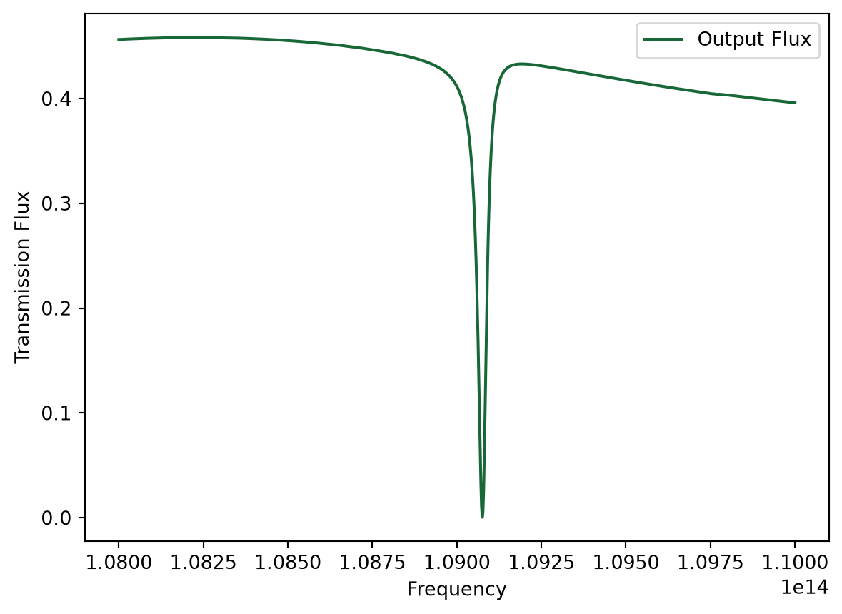
Compute Resonance Frequency and Q
We import Tidy3D’s resonance finder
from tidy3d.plugins.resonance import ResonanceFinder

resfinder = ResonanceFinder(freq_window=(freqs[0], freqs[-1]))
res_data = resfinder.run_scalar_field_time(signal=sim_linear_data.monitor_data["field time wg"].Ez)
res_data = res_data.sortby("error")
res_data.to_dataframe()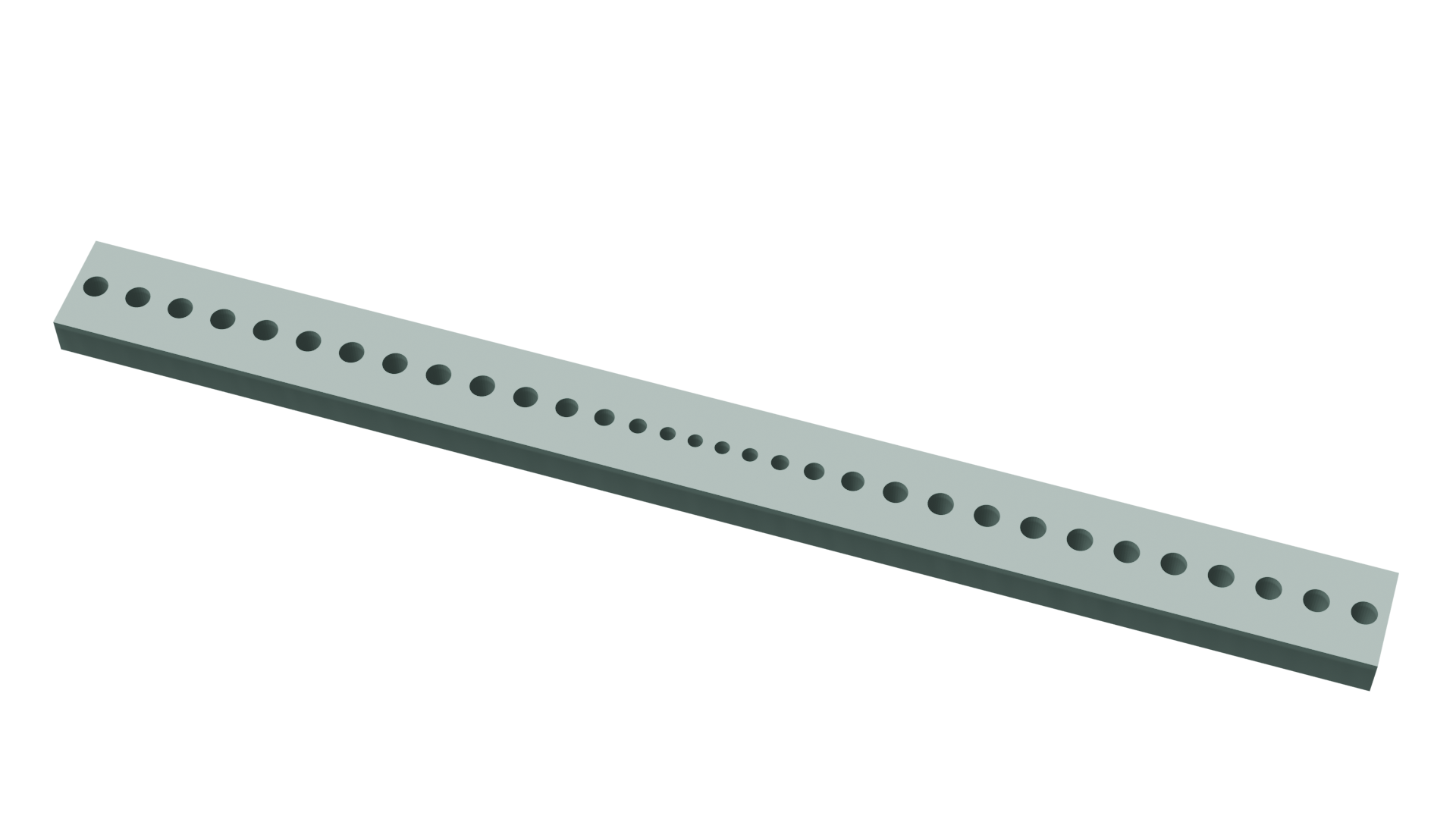
No matching results found.


 TERMS & CONDITIONS


 How the process works:
 Try this real URL to see an example: