





Author: Xinyi Wang, Texas A&M University
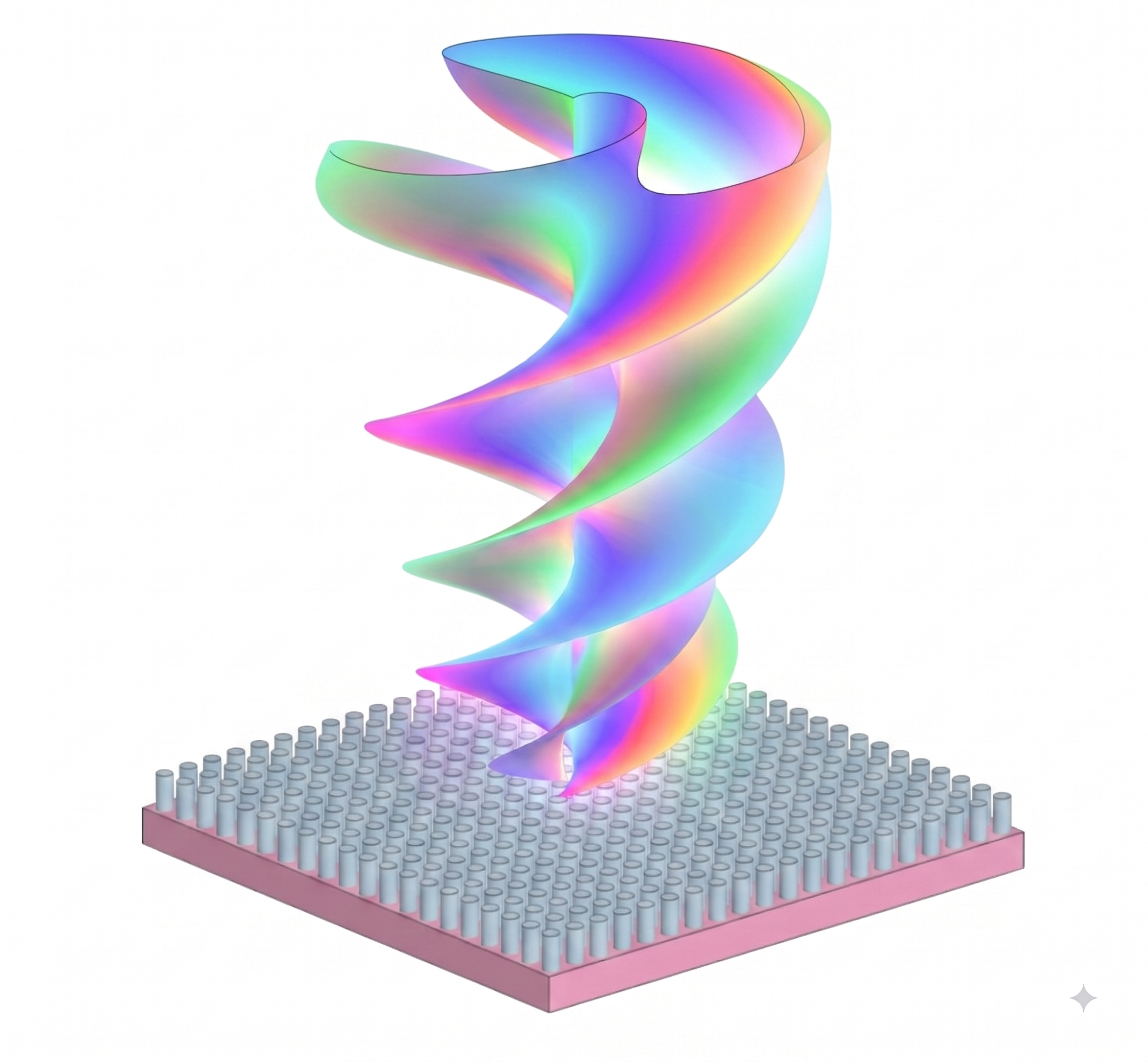
This notebook demonstrates a dielectric metasurface supporting a bound state in the continuum (BIC) with a vortex-like far-field response. It builds the periodic structure, illuminates it with circularly polarized light, and analyzes the resulting phase and orbital angular momentum content in momentum space.
The example is intended to show how to combine geometry construction, far-field projection, and post-processing to characterize polarization-dependent vortex behavior in a photonic metasurface.
# imported libraries
import tidy3d as td
import numpy as np
from tidy3d import web
import matplotlib.pyplot as plt
from warnings import warn
from matplotlib.colors import Normalize
from scipy.special import genlaguerre
import math

# Creating the metasurface
n_length = 20 # number of holes length-wise
n_width = 20  # number of holes width-wise

# metasurface uses Si3N4 dielectric
index_sub = 1.46 # index of refraction for the substrate

lattice_constant = 0.41  # spacing between the pillars on the metasurface
radius_pillars = 0.12      # radius of the pillars
thickness_ms = 0.5     # thickness of the pillars
thickness_sub = 0.5      # thickness of the substrate

ms_length = (n_length - 1) * lattice_constant + 2 * radius_pillars   # length of the metasurface
ms_width = (n_width - 1) * lattice_constant + 2 * radius_pillars   # width of the metasurface

Wl = 0.91  # wavelength of the input light

projdist = 250 * Wl #changes the projdist for in-sim farfieldmonitor object, doesn't do much. Change the r_proj in the postprocessing stage to change the projection distance for the inteference pattern

#defines the distance from gaussian beam source to metasurface and adjusts simulation accordingly
ms_monitor_gap = Wl * 2
simheight = 0.2 + thickness_ms + thickness_sub + ms_monitor_gap

#For obtaining good simulation results, tuning the waist distance and projection distance below are critical.

print(ms_length, ms_width)
8.03 8.03
Simulation Setup
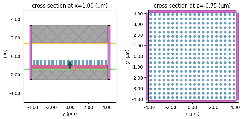
This section defines the dielectric metasurface geometry: a periodic array of silicon nitride pillars on a substrate. The resulting pattern sets the resonant lattice that supports the bound-state-in-the-continuum response.
# Creating the Metasurface
def slab_square_array(
    x0,
    y0,
    z0,
    R,
    hole_spacing_x,
    hole_spacing_y,
    n_x,
    n_y,
    height,
    pillar_medium,
    reference_plane="bottom",
    sidewall_angle=0,
    axis=2,
):
    # parameters
    # ------------------------------------------------------------
    # x0: x coordinate of center of the array (um)
    # y0: y coordinate of center of the array (um)
    # z0: z coordinate of center of the array (um)
    # R: radius of the circular holes (um)
    # hole_spacing_x: distance between centers of holes in x direction (um)
    # hole_spacing_y: distance between centers of holes in y direction (um)
    # n_x: number of holes in x direction
    # n_y: number of holes in y direction
    # height: height of array
    # pillar_medium: medium of the holes
    # reference_plane
    # sidewall_angle: angle slant of cylinders. Add compensation for the box geometry if != 0?
    # axis

    start_x, start_y = x0 - hole_spacing_x * (n_x - 1) / 2, y0 - hole_spacing_y * (n_y - 1) / 2
#(hole_spacing_x * n_x, hole_spacing_y * n_y, height)
    # box = td.Box(center=(x0, y0, simheight/2 - 4 + z0), size=(td.inf,td.inf,height))
    structures = []
    cylinders = []

    for i in range(0, n_x):
        for j in range(0, n_y):
            c = td.Cylinder(
                axis=axis,
                sidewall_angle=sidewall_angle,
                reference_plane=reference_plane,
                radius=R,
                center=(start_x + i * hole_spacing_x, start_y + j * hole_spacing_y, z0),
                length=height,
            )
            cylinders.append(c)

    cylinders_structure = td.Structure(
        geometry=td.GeometryGroup(geometries=cylinders), medium=pillar_medium, name = "Pillars"
    )

    structures.append(cylinders_structure)

    return structures

ms = slab_square_array(
    0,
    0,
    thickness_ms / 2 + thickness_sub + 0.1 - simheight / 2,
    radius_pillars,
    lattice_constant,
    lattice_constant,
    n_length,
    n_width,
    thickness_ms,
    td.material_library['cSi']['Green2008'] ,
)

# Creating the Substrate
    # Glass Substrate: Permittivity = 1.5, Thickness = 2
substrate = td.Structure(geometry = td.Box(center = (0, 0,-simheight / 2 + 0.1 + thickness_sub / 2),
                                            size = (td.inf, td.inf, thickness_sub)),
                        medium = td.Medium(permittivity = index_sub**2),
                        name = "Substrate")

# # Creating the Mesh
mesh_override = td.MeshOverrideStructure(
    geometry=td.Box(center=(0, 0, thickness_ms / 2 + thickness_sub + 0.1 - simheight / 2), size=(ms_length, ms_width, thickness_ms)),
    dl=(0.01,) * 3,
)

# # Creating a Vacuum Object
# vac = td.Structure(geometry = td.Box(center = (0,0,0), size = (1,1,1)),
#                    medium = td.Medium.from_nk(n = 1, k = 0, freq = 0.4),
#                    name = "Empty Box")
This cell creates the circularly polarized Gaussian source and the corresponding near-field and far-field monitors used to measure the response of the metasurface.
# Creating a Circular Light Source
size_source = (td.inf, td.inf, 0)
fcen = td.C_0 / Wl # defining the central frequency
fwidth = 0.01 * fcen # defining the linewidth of the source
deg = 0 * np.pi / 180 #Incident angle of the circularly-polarized source
w_dist = 50 * Wl   #distance of the beam waist from bottom of the PhC
def circular_polarized_plane_wave(pol):
    # define a plane wave polarized in the x direction
    plane_wave_x = td.GaussianBeam(
        source_time=td.GaussianPulse(freq0 = fcen, fwidth = fwidth),
        size=size_source,
        center=(0, 0,-simheight / 2 + 0.1),
        direction="+",
        pol_angle=0,
        angle_theta = deg,
        waist_distance = w_dist
        #,waist_radius=4 * Wl
    )
    # determine the phase difference given the polarization
    if pol == "left":
        phase = -np.pi / 2
    elif pol == "right":
        phase = np.pi / 2
    else:
         warn("pol must be `left` or `right`")
    # define a plane wave polarized in the y direction with a phase difference
    plane_wave_y = td.GaussianBeam(
        source_time=td.GaussianPulse(freq0 = fcen, fwidth = fwidth, phase = phase),
        size=size_source,
        center=(0, 0,-simheight / 2 + 0.1),
        direction="+",
        pol_angle=np.pi / 2,
        angle_theta = deg,
        waist_distance = w_dist
        #,waist_radius = 4 * Wl
    )
    return [plane_wave_x, plane_wave_y]

polarization = "left"
source = circular_polarized_plane_wave(polarization)

# Creating the Monitors
out_Wl = Wl
out_fcen = td.C_0 / out_Wl

far_field_monitor = td.FieldProjectionCartesianMonitor(
    center=(0, 0, simheight / 2 - 0.1),
    size=(td.inf, td.inf, 0),
    normal_dir="+",
    freqs=out_fcen,
    x=ms_length * 2.5 * np.linspace(-0.5, 0.5, 100),  # changed from 5  6/24/2025 2:30 PM
    y=ms_length * 2.5 * np.linspace(-0.5, 0.5, 100),  # changed from 5
    proj_axis=2,
    proj_distance=projdist,
    far_field_approx=False,
    name="farFieldMon",
)

field_monitor = td.FieldMonitor(
    center=far_field_monitor.center,
    size=far_field_monitor.size,
    freqs=far_field_monitor.freqs,
    name="fieldMon",
    colocate = False,
)

k_space_monitor = td.FieldProjectionKSpaceMonitor(
    center = far_field_monitor.center,
    size = far_field_monitor.size,
    name = "kSpaceMon",
    colocate = True,
    freqs = far_field_monitor.freqs,
    far_field_approx = False,
    proj_axis = 2,
    proj_distance = projdist,
    ux = list(np.linspace(-1, 1, 100)),
    uy = list(np.linspace(-1, 1, 100)),
)
This cell assembles the full Tidy3D simulation, including the materials, sources, boundaries, and run-time settings needed to model the metasurface response.
# Defines the Simulation
run_time = 0.75e-12
sim = td.Simulation(
    size = (ms_length+(lattice_constant - 2 * radius_pillars), ms_width+(lattice_constant - 2 * radius_pillars), simheight),
    grid_spec=td.GridSpec.auto(
        min_steps_per_wvl = 10,
        override_structures = [mesh_override],
    ),
    structures = ms + [substrate],
    sources = source,
    monitors = [field_monitor, k_space_monitor],
    run_time = run_time,
    # boundary_spec=td.BoundarySpec(
    #     x = td.Boundary.pml(num_layers=12), y = td.Boundary.pml(num_layers=12), z = td.Boundary.pml(num_layers=12)
    # ),
    boundary_spec=td.BoundarySpec(
            x = td.Boundary.bloch_from_source(source=source[0], domain_size=ms_length+(lattice_constant - 2 * radius_pillars), axis=0, medium = td.Medium(permittivity = 1**2)),
            y = td.Boundary.bloch_from_source(source=source[1], domain_size=ms_width+(lattice_constant - 2 * radius_pillars), axis=0, medium = td.Medium(permittivity = 1**2)),
            z = td.Boundary.absorber(num_layers = 20),
        ),
    shutoff = 0,
    medium = td.Medium(permittivity = 1),
)
sim.plot_3d()
print(sim.num_cells/100000000, sim.num_time_steps/50000)
def check_simulation_and_generate_message(sim):
    if sim.num_cells < 100_000_000 and sim.num_time_steps < 50_000:
        return "can run this simulation for free"
    return "conditions not met"

# Example usage
result = check_simulation_and_generate_message(sim)
print(result)

fig, Ax = plt.subplots(1, 2, tight_layout=True, figsize=(8, 3.8))

sim.plot(x=1, ax=Ax[0])
# mesh.plot(x=1, ax=Ax[0], alpha=0.2)
Ax[0].set_xlim(-5, 5)
Ax[0].set_ylim(-5, 5)
Ax[1].set_xlim(-1, 1)
Ax[1].set_ylim(-3, 3)

sim.plot(z = -0.75, ax = Ax[1])
plt.show()
0.8634925 0.8356
can run this simulation for free
# estimating the credit cost of the simulation
task_id = web.upload(sim, task_name = "vortexMetasurface")
web.estimate_cost(task_id)
11:55:44 EDT Created task 'vortexMetasurface' with resource_id
             'fdve-10a957c2-67b3-422b-87a3-9689c125744d' and task_type 'FDTD'.
             View task using web UI at
             'https://tidy3d.simulation.cloud/workbench?taskId=fdve-10a957c2-67b
             3-422b-87a3-9689c125744d'.
Task folder: 'default'.
Output()
11:55:47 EDT Estimated FlexCredit cost: 4.667. Minimum cost depends on task
             execution details. Use 'web.real_cost(task_id)' to get the billed
             FlexCredit cost after a simulation run.
11:55:48 EDT Estimated FlexCredit cost: 4.667. Minimum cost depends on task
             execution details. Use 'web.real_cost(task_id)' to get the billed
             FlexCredit cost after a simulation run.
4.666704829093208
results = web.run(
    simulation = sim,
    task_name = "tdarray_simsize20x20_gaussianinput1.32",
    folder_name = "SiPillars_BIC_OV_Gen",
    path = "data/%s.hdf5" % "1",
    verbose = "True",
)
             Created task 'tdarray_simsize20x20_gaussianinput1.32' with
             resource_id 'fdve-49dcf727-8cbe-4b69-9416-4302e88556bd' and
             task_type 'FDTD'.
             View task using web UI at
             'https://tidy3d.simulation.cloud/workbench?taskId=fdve-49dcf727-8cb
             e-4b69-9416-4302e88556bd'.
Task folder: 'SiPillars_BIC_OV_Gen'.
Output()
11:55:51 EDT Estimated FlexCredit cost: 4.667. Minimum cost depends on task
             execution details. Use 'web.real_cost(task_id)' to get the billed
             FlexCredit cost after a simulation run.
11:55:52 EDT status = success
Output()
11:56:04 EDT Loading simulation from data/1.hdf5
Far-field Projection Settings
This section projects the near-field response into the far field and defines the reciprocal-space sampling used for the vortex and phase analysis.
# radial distance away from the origin at which to project fields

r_proj = 250 * Wl

#size of each axes of the projection window, in micro-meters

size = 250

#size of the axes of the ndarray

dimsize = 250

# here we add the 'window_size' argument to ensure that the near fields decay to zero at the monitor boundaries
far_field_local_projection = td.FieldProjectionCartesianMonitor(
    center=(0, 0, simheight / 2 - 2),
    size=(td.inf, td.inf, 0),
    normal_dir="+",
    freqs=[td.C_0 / Wl],
    x=size  * np.linspace(-0.5, 0.5, dimsize),
    y=size * np.linspace(-0.5, 0.5, dimsize),
    proj_axis=2,
    proj_distance=r_proj,
    far_field_approx=False,
    window_size=(0.08, 0.08),
    name="farFieldLocalProjection",
)

projector = td.FieldProjector.from_near_field_monitors(
    sim_data=results,
    near_monitors=[field_monitor],
    normal_dirs=["+"],
    pts_per_wavelength=10,
)
projected = projector.project_fields(far_field_local_projection)
far_field = projected.fields_cartesian
Output()
E-field Component Profiles
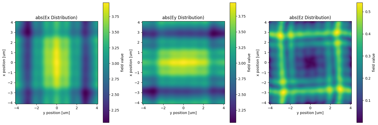
This cell visualizes the field components at the monitor plane to confirm the spatial distribution of the excited modes before extracting the circular polarization content.
# Plot the E-field distribution

fig, axs = plt.subplots(1, 3, figsize=(15, 5))

# Assuming results and fcen are defined elsewhere in your code
# Plot Ex
Ex = results['fieldMon'].Ex.sel(f=fcen).abs
Ex.plot(ax=axs[0])
axs[0].set_title('abs(Ex Distribution)')
axs[0].set_aspect('equal')

# Plot Ey
Ey = results['fieldMon'].Ey.sel(f=fcen).abs
Ey.plot(ax=axs[1])
axs[1].set_title('abs(Ey Distribution)')
axs[1].set_aspect('equal')

# Plot Ez
Ez = results['fieldMon'].Ez.sel(f=fcen).abs
Ez.plot(ax=axs[2])
axs[2].set_title('abs(Ez Distribution)')
axs[2].set_aspect('equal')

# Display the plots together
plt.tight_layout()
plt.show()
# Extract RCP and LCP components

RCP = (far_field["Ex"] - 1j * far_field["Ey"]) / np.sqrt(2)
LCP = (far_field["Ex"] + 1j * far_field["Ey"]) / np.sqrt(2)
comp = [RCP, LCP]
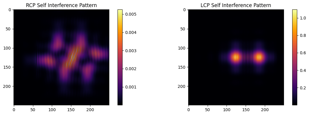
Self-interference Patterns
This cell computes and plots the self-interference pattern for the RCP and LCP components to visualize the phase winding and vortex-like structure.
# Self-interference pattern
# In practice it is easiest to shift only the x coordinate; the code also supports shifting the interfering beam in both x and y.

xshift = 60
yshift = 0
fill = 0
RCP_Left = RCP.shift(x=0, y = 0, fill_value = fill)
RCP_Right = RCP.shift(x=xshift, y = yshift, fill_value = fill)

LCP_left = LCP.shift(x=0, y = 0, fill_value = fill)
LCP_right = LCP.shift(x=xshift, y = yshift, fill_value = fill)

shifted_comps = [[RCP_Right,RCP_Left],[LCP_right,LCP_left]]

fig, axc = plt.subplots(1, 2, figsize=(12,4))
for i in range(2):
    selfpattern = (shifted_comps[i][0].squeeze().T + shifted_comps[i][1].squeeze().T) ** 2
    pos = axc[i].imshow(
        abs(
            selfpattern.squeeze()
        ),
        interpolation="bilinear",
        cmap="inferno",
        )
    if(i == 0):
        axc[i].set_title("RCP Self Interference Pattern")
    else:
        axc[i].set_title("LCP Self Interference Pattern")
    axc[i].axis("on")
    fig.colorbar(pos,ax=axc[i])

plt.tight_layout()
plt.show()
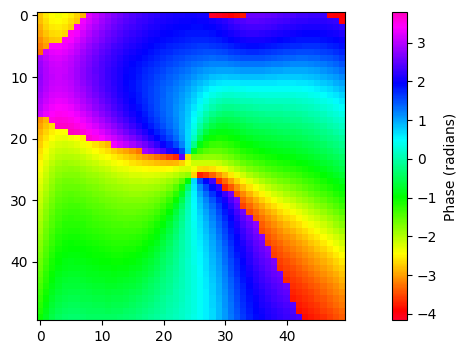
Phase Profile of Circularly Polarized Components
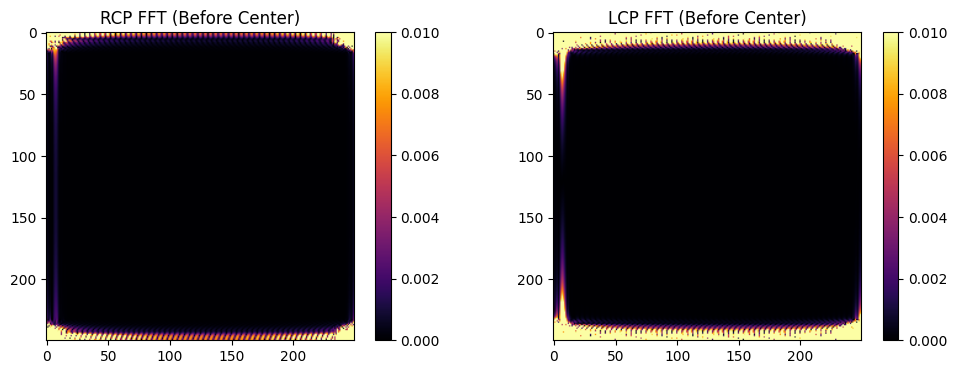
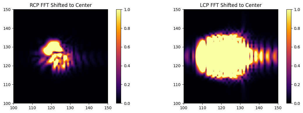
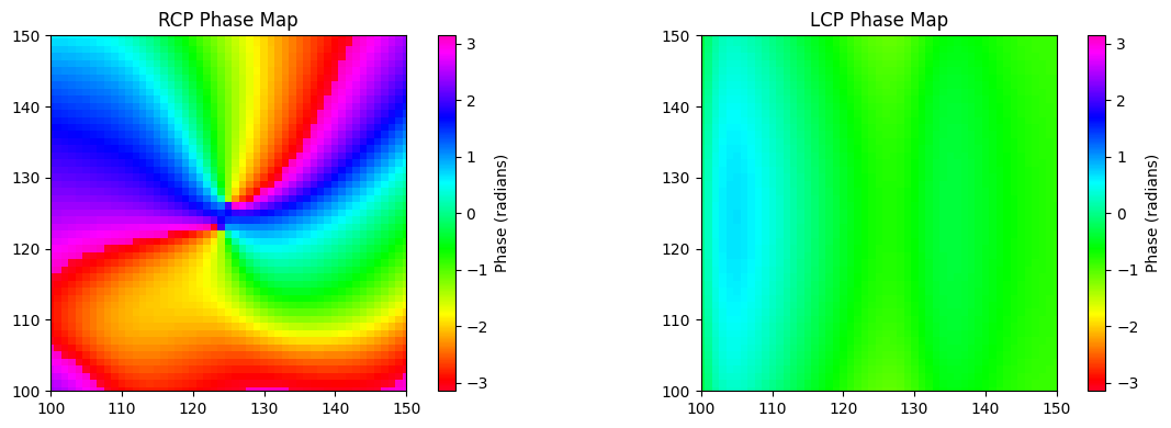
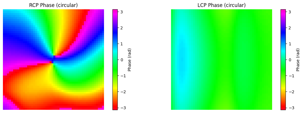
This section centers the Fourier-domain spot, reconstructs the phase map for each circular polarization, and plots the result to identify the helical phase profile.
x = np.linspace(- size / 2, size / 2, dimsize)
y = np.linspace(- size / 2, size / 2, dimsize)
X, Y = np.meshgrid(x, y)
r = np.sqrt(X**2 + Y**2)

# To center the "bright spot" in k-space and retrieve the phase profile, there are two options:
# 1. Adjust the k_vec variable below
# 2. Roll the numpy array to center the spot
#
#Theoretically, the first option allows for finer tuning and cleaner results, but in practice there has not been much difference. Regardless, both are available.
#If wanting to use the first option, leave k_vec non-zero, and comment the lines marked "COMMENT/UNCOMMENT HERE"
#If wanting to use the second, set k_vec to be zero, uncomment the aforementioned lines

k_vec = 1.64

I_RCP = shifted_comps[0][0].T * np.conjugate(shifted_comps[0][1].T)
I_RCP = I_RCP.dropna(dim = 'x')
I_RCP *= np.exp(x * k_vec * 1j)
FFT_before_RCP = np.fft.fft2(I_RCP)

I_LCP = shifted_comps[1][0].T * np.conjugate(shifted_comps[1][1].T)
I_LCP = I_LCP.dropna(dim='x')
I_LCP *= np.exp(x * k_vec * 1j)
FFT_before_LCP = np.fft.fft2(I_LCP)

I_comp = [I_RCP,I_LCP]

FFT_arr = [FFT_before_RCP, FFT_before_LCP]

# fig, axp = plt.subplots(1, 2, figsize=(12,4))
# for i in range(2):
#     pos = axp[i].imshow(
#         abs(
#             I_comp[i].squeeze()
#         ),
#         interpolation="bilinear",
#         cmap="inferno",
#     )
#     if(i == 0):
#         axp[i].set_title("I (RCP)")
#     else:
#         axp[i].set_title("I (LCP)")
#     fig.colorbar(pos, ax=axp[i])

fig, axp = plt.subplots(1, 2, figsize=(12,4))
for i in range(2):
    pos = axp[i].imshow(
        abs(
            FFT_arr[i].squeeze()
        ),
        interpolation="bilinear",
        cmap="inferno",
        norm=Normalize(vmin=0, vmax=0.01) #change vmax to change colorbar's scale
    )
    if(i == 0):
        axp[i].set_title("RCP FFT (Before Center)")
    else:
        axp[i].set_title("LCP FFT (Before Center)")
    axp[i].axis("on")

    #uncomment/comment below to zoom in/out of the center

    # axp[i].set_xlim([110,140])
    # axp[i].set_ylim([110,140])
    fig.colorbar(pos, ax=axp[i])

# Shift FFT for easier visualization
FFT_shift_RCP = np.fft.fftshift(FFT_before_RCP.squeeze())
FFT_shift_LCP = np.fft.fftshift(FFT_before_LCP.squeeze())

#Approximately determine the largest magnitude point in k-space

highest = 0
maxima_x = 0
maxima_y = 0

for i in range(dimsize):
    for j in range(dimsize):
        if(np.abs(FFT_shift_RCP[i][j]) > highest):
            maxima_x = j
            maxima_y = i
            highest = FFT_shift_RCP[i][j]

print(maxima_x,maxima_y)

middle = math.floor(size / 2)
xshift = middle - maxima_x + (-2)
yshift = middle - maxima_y + 4

#Adjust the highest magnitude to be the center
#IMPORTANT: More likely than not, you will have to adjust how much the code shifts the data manually to get the "bright spot" as close to the center as possible

#COMMENT/UNCOMMEN THIS LINE
# FFT_shift_RCP = np.roll(FFT_shift_RCP,(xshift,yshift), axis = (1,0))

#Ditto for LCP

highest = 0
maxima_x = 0
maxima_y = 0

for i in range(dimsize):
    for j in range(dimsize):
        if(np.abs(FFT_shift_LCP[i][j]) > highest):
            maxima_x = j
            maxima_y = i
            highest = FFT_shift_LCP[i][j]

# print(maxima_x,maxima_y)

#COMMENT/UNCOMMENT THIS LINE
# FFT_shift_LCP = np.roll(FFT_shift_LCP,(xshift,yshift), axis = (1,0))

FFT_shift_arr = [FFT_shift_RCP, FFT_shift_LCP]
approx_size = 50    #how large the diameter of the RCP pattern appears to be
hi = middle + math.floor(approx_size/2)
lo = middle - math.floor(approx_size/2)
fig, axp = plt.subplots(1, 2, figsize=(12, 4))
for i in range(2):
    pos = axp[i].imshow(
        np.abs(FFT_shift_arr[i]),
        interpolation="bilinear",
        cmap="inferno",
        norm=Normalize(vmin=0, vmax = 1) #change vmax to change colorbar's scale
    )
    if i == 0:
        axp[i].set_title("RCP FFT Shifted to Center")
    else:
        axp[i].set_title("LCP FFT Shifted to Center")
    axp[i].axis("on")
    fig.colorbar(pos, ax=axp[i])
    axp[i].set_xlim([lo,hi])
    axp[i].set_ylim([lo,hi])

plt.tight_layout()
plt.show()

#Shift the FFT array back so that the computer can do math on it and perform an inverse fourier transform

retrieved_field_RCP = np.fft.ifft2(np.fft.ifftshift(FFT_shift_RCP))
retrieved_field_LCP = np.fft.ifft2(np.fft.ifftshift(FFT_shift_LCP))

#Retrieve the phase from the inverse fourier transform

phase_map_RCP = np.angle(retrieved_field_RCP)
phase_map_LCP = np.angle(retrieved_field_LCP)
phase_map = [phase_map_RCP, phase_map_LCP]

fig, axp = plt.subplots(1, 2, figsize=(12, 4))
for i in range(2):
    pos = axp[i].imshow(
        phase_map[i],
        cmap="gist_rainbow",
        # interpolation="bilinear"
    )
    if i == 0:
        axp[i].set_title("RCP Phase Map")
    else:
        axp[i].set_title("LCP Phase Map")
    axp[i].axis("on")
    fig.colorbar(pos, ax=axp[i], label="Phase (radians)")

    #uncomment/comment below to zoom in/out of the center

    axp[i].set_xlim([lo,hi])
    axp[i].set_ylim([lo,hi])
plt.tight_layout()
plt.savefig("Phase_plot.svg", format="svg")
plt.show()
124 132
# Circular mask settings
# use the same crop window [lo:hi] you're already plotting
Xc = X[lo:hi, lo:hi]
Yc = Y[lo:hi, lo:hi]
rc = np.sqrt(Xc**2 + Yc**2)

R = rc.max()  # or pick a physical radius you want (same units as x,y)
circle_mask = rc <= R

# Mask phase outside the circle
phase_map_RCP_c = np.where(circle_mask, phase_map_RCP[lo:hi, lo:hi], np.nan)
phase_map_LCP_c = np.where(circle_mask, phase_map_LCP[lo:hi, lo:hi], np.nan)

phase_map_c = [phase_map_RCP_c, phase_map_LCP_c]

fig, axp = plt.subplots(1, 2, figsize=(12, 4))
for i in range(2):
    pos = axp[i].imshow(
        phase_map_c[i],
        cmap="gist_rainbow",
        origin="lower",
        vmin=-np.pi, vmax=np.pi
    )
    axp[i].set_title("RCP Phase (circular)" if i == 0 else "LCP Phase (circular)")
    axp[i].axis("off")
    fig.colorbar(pos, ax=axp[i], label="Phase (rad)")

plt.tight_layout()
# plt.savefig("Phase_plot_circular.svg", format="svg")
plt.show()
Polarization Vector Plot
#retrieve orientation angle of the polarization vectors, plot
phase_RCP = phase_map_RCP[lo:hi,lo:hi]
phase_LCP = phase_map_LCP[lo:hi,lo:hi]

psi = phase_LCP - phase_RCP

fig, axp = plt.subplots(1, 1, figsize=(12, 4))
pos = axp.imshow(
    psi,
    cmap="gist_rainbow",
)

axp.axis("on")
fig.colorbar(pos, ax=axp, label="Phase (radians)")
<matplotlib.colorbar.Colorbar at 0x11dd9c7d0>
OAM Purity Analysis
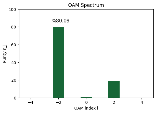
This cell evaluates the orbital angular momentum content by projecting the field onto Laguerre-Gaussian modes and plotting the resulting OAM spectrum.
def lg_mode(p, l, r, phi, w0):
    first = np.sqrt(2 * math.factorial(p) / (np.pi * w0**2 * math.factorial(p + abs(l))))
    second = (np.sqrt(2) * r / w0)**abs(l)
    third = genlaguerre(p, abs(l))  ( (np.sqrt(2) * r / w0)**2 )
    fourth = np.exp(-1 * second**2 / 2)
    fifth = np.exp(-1j * l * phi)
    return first * second * third * fourth * fifth

def inner_product(E, LG, dr, dphi, r):
    # ⟨LG | E⟩ using integration
    return np.sum(np.conjugate(LG) * E * r) * dr * dphi


def compute_Cl2_for_l(E, r, phi, w0, l, p_max, dr, dphi):
    # C_l^2 = sum over p of |<LG_{p,l} | E>|^2.
    sum_p = 0.0
    for p in range(p_max + 1):
        LG = lg_mode(p, l, r, phi, w0)
        Cp_l = inner_product(E, LG, dr, dphi, r)
        sum_p += np.abs(Cp_l)**2
    return sum_p


def compute_oam_purity(E, r, phi, w0, l_vals, p_max=10):
    # n_l
    dr = r[1, 0] - r[0, 0]
    dphi = phi[0, 1] - phi[0, 0]

    Cl2 = [compute_Cl2_for_l(E, r, phi, w0, l, p_max, dr, dphi) for l in l_vals]
    Cl2 = np.array(Cl2)

    eta = Cl2 / np.sum(Cl2)  # normalize
    return eta

# sx = dimsize / 2
sx = hi - middle
# sy = dimsize / 2
sy = hi - middle

#Starting from here, the below is vestigial code remaining that will allow you to perform the OAM purity analysis on the LP components. You'll have to uncomment and move things back to do so

# Ex_c = results['fieldMon'].Ex.sel(f=fcen).values
# Ey_c = results['fieldMon'].Ey.sel(f=fcen).values
# Ez_c = results['fieldMon'].Ez.sel(f=fcen).values
# # Ex_c = far_field['Ex']
# # Ey_c = far_field['Ey']
# # Ez_c = far_field['Ez']

# phase_Ex = np.angle(Ex_c)
# phase_Ey = np.angle(Ey_c)
# phase_Ez = np.angle(Ez_c)

# E_total = Ex_c + Ey_c + Ez_c

# # Simulation Dimensions
# # ny, nx, nz = Ex_c.shape
# # ny, nx, nz = (size,size,size)

# reduced_Etotal = np.squeeze(E_total[lo:hi,lo:hi])
# reduced_phase = np.squeeze(phase_map[0][lo:hi,lo:hi])

# Amplitude, Phase, and Measured Efield
# amplitude_array = np.sqrt(np.abs(np.squeeze(reduced_Etotal))**2)
# # phase_array = np.angle(E_total)
# Efield = amplitude_array * np.exp(1j * np.squeeze(reduced_phase))

# END

#For our purposes, we perform the OAM purity analysis only on each of the circularly polarized components of the generated light


#change LCP to RCP and vice versa to perform analysis on different CP component
reduced_CP = np.squeeze(RCP[lo:hi,lo:hi])

ny, nx, nz = (hi-lo,hi-lo,size)

w0 = 250 #need to manually adjust this parameter per simulation, should be roughly equal to the approx_size variable

x = np.linspace(-sx, sx, nx)
y = np.linspace(-sy, sy, ny)
X, Y = np.meshgrid(x, y)
r = np.sqrt(X**2 + Y**2)
phi = np.arctan2(Y, X)

# Compute OAM purity and Plot
l_vals = np.arange(-4, 5)
eta_l = compute_oam_purity(np.squeeze(reduced_CP), r, phi, w0, l_vals)
eta_l = eta_l * 100

plt.figure(figsize=(6,4))
plt.bar(l_vals, eta_l)
plt.xlabel("OAM index l")
plt.ylabel("Purity η_l")
plt.title("OAM Spectrum")
plt.ylim(0, 100)
plt.text(np.argmax(eta_l) - len(l_vals) / 2, eta_l[np.argmax(eta_l)] + 5, "%" + f'{eta_l[np.argmax(eta_l)]:.2f}', fontsize=12)
plt.show()
Interference Patterns and Intensity Profiles
#Generate intensity profiles, interference patterns

xmin = -(size/2)
xmax = size / 2

# Gaussian beam function
def E(r, z, lda=1, E0=1, w0=1, n=1):
    k = 2 * np.pi / lda
    zr = np.pi * w0**2 * n / lda
    wz = w0 * np.sqrt(1 + (z / zr) ** 2)
    Rz = z * (1 + (zr / z) ** 2)
    phi = np.arctan(z / zr)

    return (
        E0
        * (w0 / wz)
        * np.exp(-(r**2) / (wz**2))
        * np.exp(-1j * (k * z + k * r**2 / (2 * Rz) - phi))
    )

cmap = "Greys_r" #"inferno"
# Creating the data points
x = np.linspace(xmin, xmax, size)
y = x.copy()

X, Y = np.meshgrid(x, y)
r = np.sqrt(X**2 + Y**2)

# Creating the Gaussian beam field
gb = E(r, 1, Wl, w0= 100)

# Plotting the interference pattern
fig, axs = plt.subplots(1, 3, figsize=(12,4))
Ef = ["Ex", "Ey", "Ez"]  # Field components to plot

#Interference patterns of LP components with a LP Gaussian beam

for i in range(3):
    axs[i].imshow(
        abs(
            far_field[Ef[i]].squeeze().T
            / far_field[Ef[i]].max()
            + gb
        ),
        interpolation="bilinear",
        cmap=cmap ,
        )
    axs[i].set_title(f"{Ef[i]} Interference Pattern (LP Incident)")
    axs[i].axis("on")
    fig.colorbar(pos,ax=axs[i])

#Interference patterns of CP components with a LP Gaussian beam

fig, axcx = plt.subplots(1, 2, figsize=(12,4))
for i in range(2):
    pos = axcx[i].imshow(
        abs(
            comp[i].squeeze().T
            / comp[i].max()
            + gb
        ),
        interpolation="bilinear",
        cmap=cmap ,
        )
    if(i == 0):
        axcx[i].set_title("RCP Component Interference Pattern (LP Incident)")
    else:
        axcx[i].set_title("LCP Component Interference Pattern (LP Incident)")
    axcx[i].axis("on")
    fig.colorbar(pos,ax=axcx[i])

# Gaussian beam function, circularly polarized
def cpE(r, z, lda=1, E0=1, w0=1, n=1):
    k = 2 * np.pi / lda
    zr = np.pi * w0**2 * n / lda
    wz = w0 * np.sqrt(1 + (z / zr) ** 2)
    Rz = z * (1 + (zr / z) ** 2)
    phi = np.arctan(z / zr)

    gb = (E0
        * (w0 / wz)
        * np.exp(-(r**2) / (wz**2))
        * np.exp(-1j * (k * z + k * r**2 / (2 * Rz) - phi)))

    cpEx = gb / np.sqrt(2)
    cpEy = 1j * gb / np.sqrt(2)

    return (cpEx, cpEy)

# Creating the CP Gaussian beam field
gb = cpE(r, 1 , Wl , w0=50)

#Interference patterns of LP components with a CP Gaussian beam

fig, ax = plt.subplots(1, 2, figsize=(12,4))

for i in range(2):
    pos = ax[i].imshow(
        abs(
            far_field[Ef[i]].squeeze().T
            / far_field[Ef[i]].max()
            + gb[i]
        ),
        interpolation="bilinear",
        cmap=cmap ,
        )
    ax[i].set_title(f"{Ef[i]} Interference Pattern (CP Incident)")
    ax[i].axis("on")
    fig.colorbar(pos,ax=ax[i])

#Interference patterns of CP components with a CP Gaussian beam

fig, axc = plt.subplots(1, 2, figsize=(12,4))
for i in range(2):
    pos = axc[i].imshow(
        abs(
            comp[i].squeeze().T
            / comp[i].max() +
             gb[i]
        ),
        interpolation="bilinear",
        cmap=cmap ,
        )
    if(i == 0):
        axc[i].set_title("RCP Component Interference Pattern (CP Incident)")
    else:
        axc[i].set_title("LCP Component Interference Pattern (CP Incident)")
    axc[i].axis("on")
    fig.colorbar(pos,ax=axc[i])
plt.tight_layout()
# plt.savefig("Interference_plots.svg", format="svg")

#Intensity profile of the CP components of the generated OV

fig, axcs = plt.subplots(1, 2, figsize=(12,4))
for i in range(2):
    pos = axcs[i].imshow(
        abs(
            comp[i].squeeze()
        ) ** 2,
        interpolation="bilinear",
        cmap=cmap ,
        )
    if(i == 0):
        axcs[i].set_title("RCP Intensity Profile")
    else:
        axcs[i].set_title("LCP Intensity Profile")
    axc[i].axis("on")
    fig.colorbar(pos,ax=axcs[i])
plt.tight_layout()
# plt.savefig("intensity_plots.svg", format="svg")
plt.show()
/var/folders/qn/syhrzy8n7930sgqvxv2x65s40000gn/T/ipykernel_40607/1574055690.py:50: UserWarning: Adding colorbar to a different Figure <Figure size 1200x400 with 2 Axes> than <Figure size 1200x400 with 4 Axes> which fig.colorbar is called on.
  fig.colorbar(pos,ax=axs[i])
/var/folders/qn/syhrzy8n7930sgqvxv2x65s40000gn/T/ipykernel_40607/1574055690.py:50: UserWarning: Adding colorbar to a different Figure <Figure size 1200x400 with 2 Axes> than <Figure size 1200x400 with 5 Axes> which fig.colorbar is called on.
  fig.colorbar(pos,ax=axs[i])
/var/folders/qn/syhrzy8n7930sgqvxv2x65s40000gn/T/ipykernel_40607/1574055690.py:50: UserWarning: Adding colorbar to a different Figure <Figure size 1200x400 with 2 Axes> than <Figure size 1200x400 with 6 Axes> which fig.colorbar is called on.
  fig.colorbar(pos,ax=axs[i])
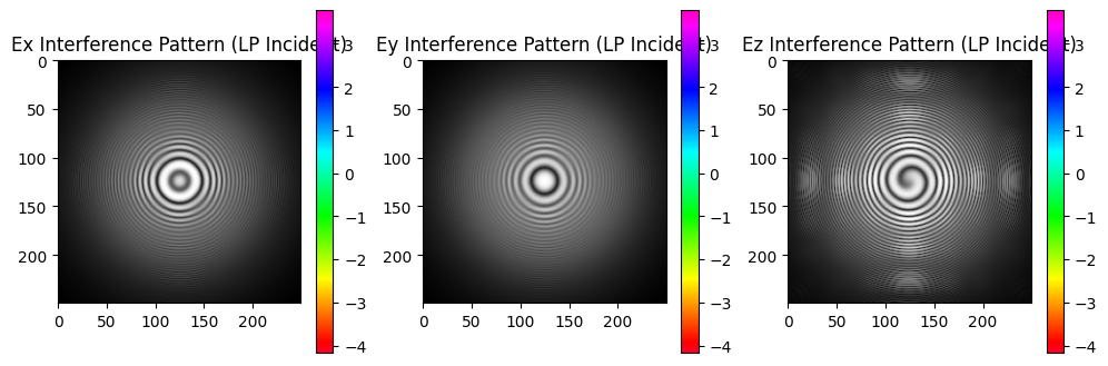
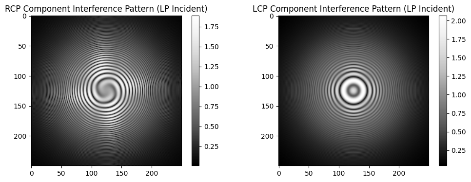
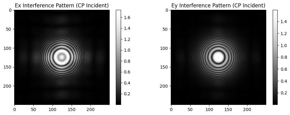
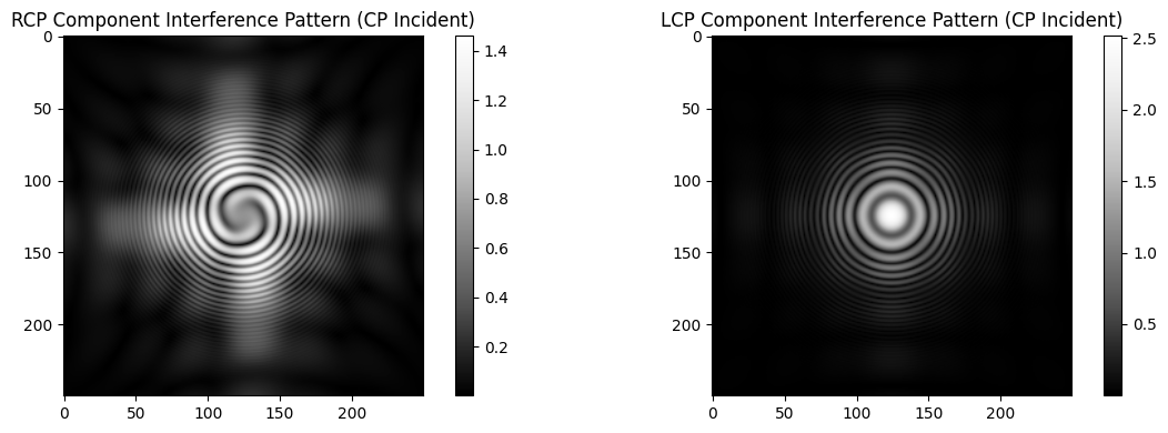
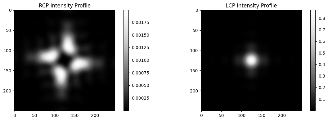
This section compares the interference and intensity patterns for the linear and circular polarization channels, highlighting how the vortex beam emerges in the generated output field.
Component Intensities in Momentum Space
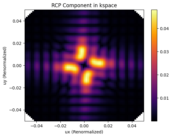
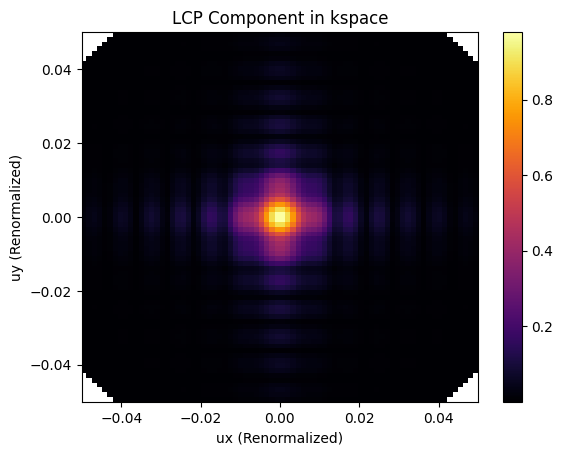
This final section visualizes the momentum-space intensity for the RCP and LCP components, confirming the directional content of the output beam in k-space.
# Plot K Space data
kspace_ux = results["kSpaceMon"].ux
kspace_uy = results["kSpaceMon"].uy

renorm_ux = kspace_ux * lattice_constant / (2 * np.pi)
renorm_uy = kspace_uy * lattice_constant / (2 * np.pi)

kresults = results["kSpaceMon"].fields_cartesian

kRCP = (kresults["Ex"] - 1j * kresults["Ey"]) / np.sqrt(2)

plt.pcolormesh(renorm_ux, renorm_uy, np.abs(kRCP.squeeze()), cmap="inferno")
plt.title('RCP Component in kspace')
plt.colorbar()
plt.xlabel("ux (Renormalized)")
plt.ylabel("uy (Renormalized)")
plt.ylim(-0.05, 0.05)
plt.xlim(-0.05, 0.05)
plt.show()

kLCP = (kresults["Ex"] + 1j * kresults["Ey"]) / np.sqrt(2)

plt.pcolormesh(renorm_ux, renorm_uy, np.abs(kLCP.squeeze()), cmap="inferno")
plt.title('LCP Component in kspace')
plt.colorbar()
plt.xlabel("ux (Renormalized)")
plt.ylabel("uy (Renormalized)")
plt.ylim(-0.05, 0.05)
plt.xlim(-0.05, 0.05)
plt.show()



 TERMS & CONDITIONS


 How the process works:
 Try this real URL to see an example: