Dynamic control of polarization states with barium titanate integrated photonic devices¶

Author: D. Krueger, L. Tian, H.G. Kim, A. Raju, A. Posadas, A. Demkov, D. Wasserman

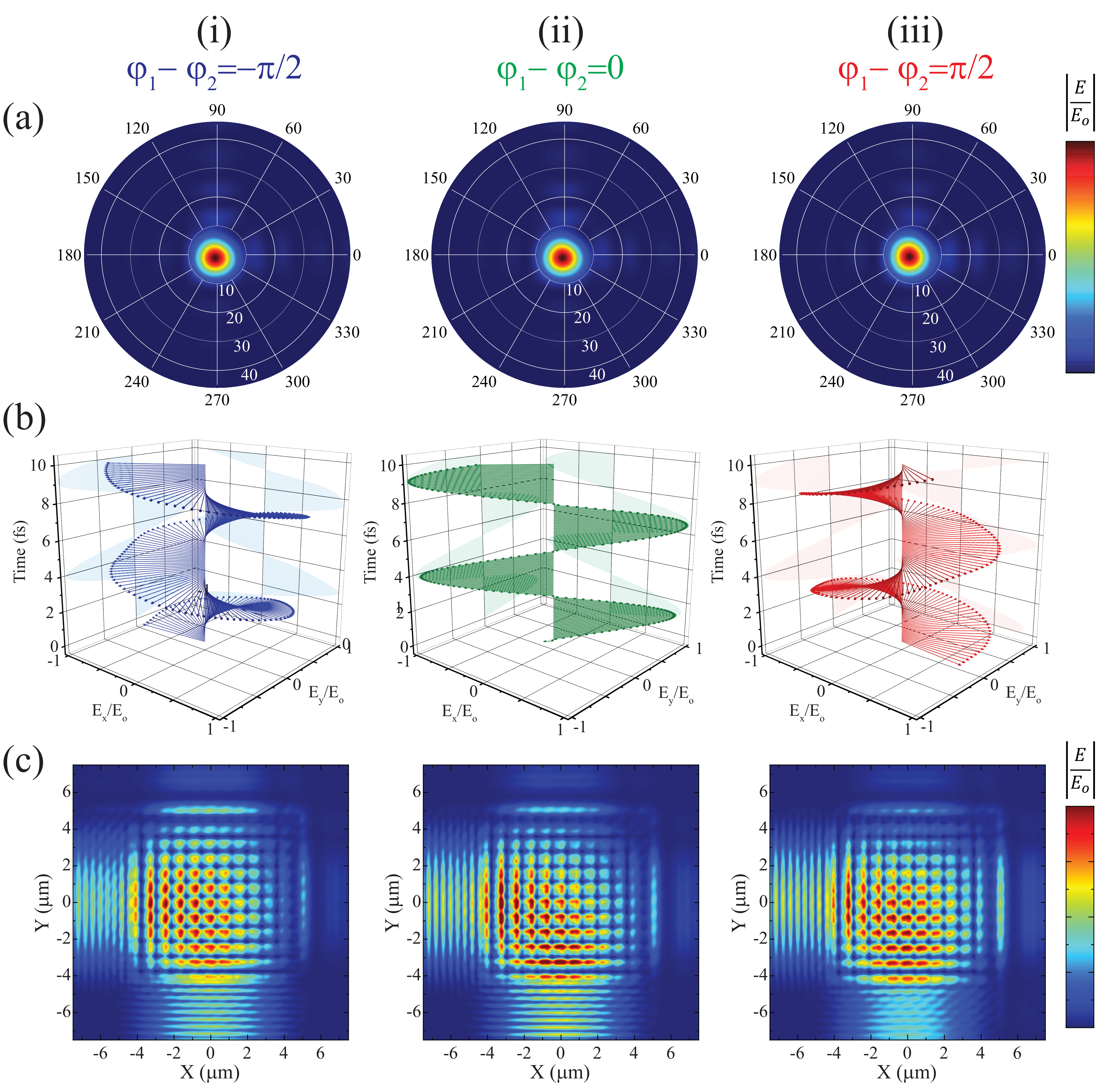
The ability to manipulate the polarization state of light is essential for a range of communication, sensing, and quantum applications. In this notebook, we demonstrate a continuous control of polarization from a two-dimensional grating outcoupler. Using Tidy3D, finite-difference time-domain (FDTD), we use different phase-shifts between two $TE_0$ mode sources to simulate Pockels effect in Mach-Zehnder interferometer. With $-\pi/2$, $0$, $\pi/2$ phase shift, we achieve polarization switching from nearly entirely left hand circularly to linearly, to nearly entirely right hand circularly polarized light.

In this notebook, we will demonstrate how to build the simulation file and show the simulation results.

[1]:

import numpy as np
import matplotlib.pyplot as plt

import tidy3d as td
import tidy3d.web as web

Simulation Configurations¶

Now we define material properties and structure geometries for the simulation:

[2]:

# Define Fixed Simulation Settings
central_wavelength = 1.55
central_freq = td.C_0 / central_wavelength
unit_spacing = 0.12
x_domain_size = unit_spacing * 10
y_domain_size = 0.3
unit_thickness = 0.03
spacer_thickness = 0.05
unit_width = 0.09


width = 10
etch_thickness = 0.1
BTO_layer = 0.2
radius = 0.315
distance = 0.185
period = 2 * radius + distance

# Define Materials
n_si = 3.48  # silicon refractive index
n_sio2 = 1.44  # silicon oxide refractive index
n_bto = 2.46  # barium titanate refractive index

Vacuum = td.Medium(
    name="Vacuum",
)

BTO = td.Medium(
    name="BTO",
    permittivity=n_bto**2,
)

SiO2 = td.Medium(
    name="SiO2",
    permittivity=n_sio2**2,
)

Then, we define two $TE_0$ mode sources, and set the phase in advanced setting manually. In this work, we only care about the performance of $1550nm$ in $TE_0$ mode, so such configuration can save the simulation time.

[3]:

# Define Sources
TE0_x = td.ModeSource(
    name="TE0_x",
    center=[-10, 0, 0],
    size=[0, 12, 2],
    source_time=td.GaussianPulse(freq0=central_freq, fwidth=central_freq / 10),
    mode_spec=td.ModeSpec(),
    direction="+",
)

TE0_y = td.ModeSource(
    name="TE0_y",
    center=[0, -10, 0],
    size=[12, 0, 2],
    source_time=td.GaussianPulse(
        freq0=central_freq, fwidth=central_freq / 10, phase=-np.pi / 2
    ),
    mode_spec=td.ModeSpec(),
    direction="+",
)

Next, we add monitors to help us analyze the simulation results. In our scenario, we should make light focus on one peak as much as possible, that means we need a field projection angle monitor to see the far-field pattern. Also, circularly polarized light means the E field in orthogonal directions should have a $\pi/2$ phase difference in time domain, which indicates we need a time monitor to extract the time signal from the peak we choose.

[4]:

# Define Monitors
Field_monitor = td.FieldMonitor(
    name="Field monitor",
    center=[0, 0, 0.5],
    size=[15, 15, 0],
    freqs=[central_freq],
)

Angle_monitor = td.FieldProjectionAngleMonitor(
    name="Angle_monitor",
    center=[0, 0, 0.5],
    size=[td.inf, td.inf, 0],
    freqs=[central_freq],
    theta=np.linspace(0, np.pi, 91),
    phi=np.linspace(0, 2 * np.pi, 181),
)

Time_monitor = td.FieldTimeMonitor(
    name="Time monitor",
    center=[0, 0, 0.5],
    size=[0, 0, 0],
    start=1e-13,
    stop=1.1e-13,
)

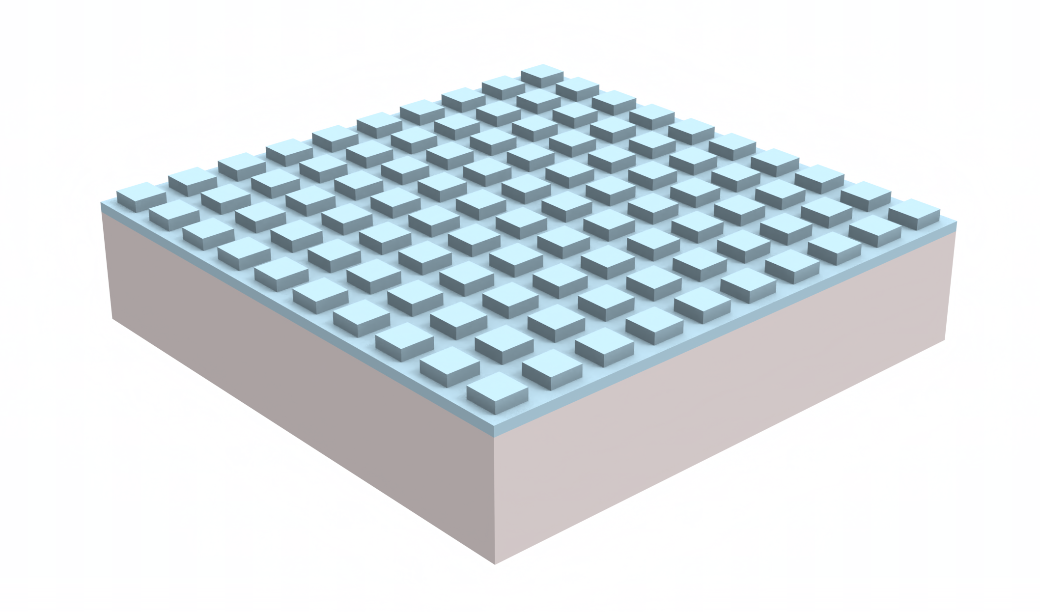
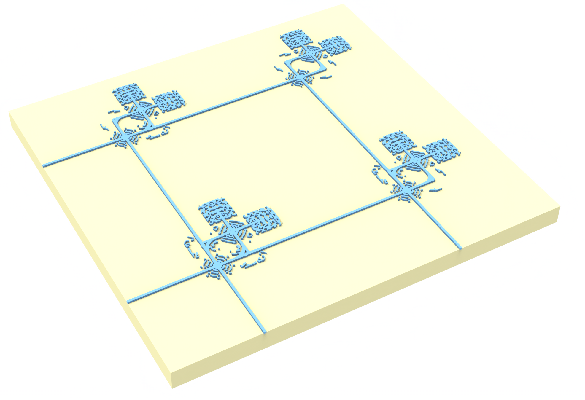
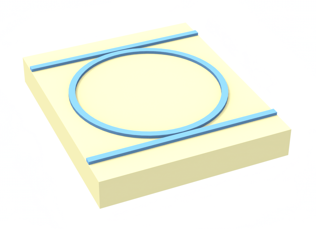
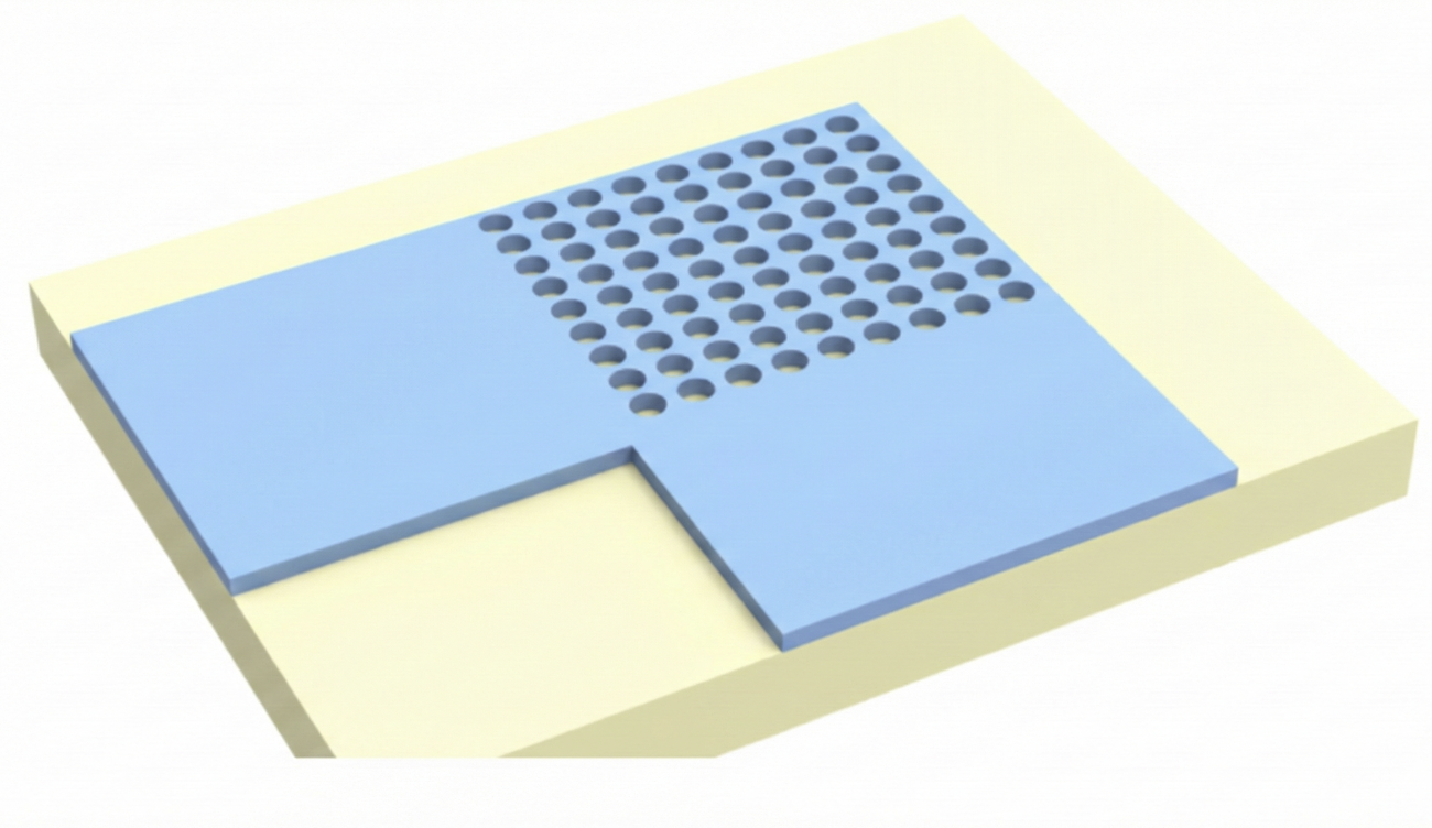
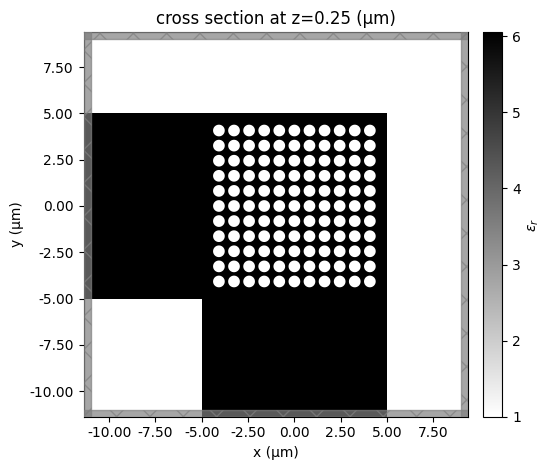
In this section, we build our structures. In this work, we choose cylinder etch array as our 2D gratings for convenienct fabrication. So in spite of two input ridge waveguides designed for $TE_0$ mode, we generate a symmetric cylinder array with vacuum medium representing etch region.

[5]:

# Define Structures

Substrate = td.Structure(
    geometry=td.Box.from_bounds(rmin=(-16, -16, -5), rmax=(14, 14, 0)),
    medium=SiO2,
)

Waveguide_1 = td.Box.from_bounds(
    rmin=(-16, -width / 2, BTO_layer),
    rmax=(-width / 2, width / 2, BTO_layer + etch_thickness),
)
Waveguide_2 = td.Box.from_bounds(
    rmin=(-width / 2, -16, BTO_layer),
    rmax=(width / 2, -width / 2, BTO_layer + etch_thickness),
)
Coupler = td.Box.from_bounds(
    rmin=(-width / 2, -width / 2, BTO_layer),
    rmax=(width / 2, width / 2, BTO_layer + etch_thickness),
)
Bottom = td.Box.from_bounds(rmin=(-16, -16, 0), rmax=(14, 14, BTO_layer))

Waveguide = td.Structure(
    name="Waveguide",
    geometry=Waveguide_1 + Waveguide_2 + Coupler + Bottom,
    medium=BTO,
)

array = []
num = int(np.floor(width / period) - 1)
half = num // 2
idx = np.arange(-half, half + 1)
for i in idx:
    for j in idx:
        cyl = td.Cylinder(
            # name = f"unit_{i}_{j}",
            center=(j * period, i * period, BTO_layer + etch_thickness / 2),
            radius=radius,
            length=etch_thickness,
            axis=2,
        )
        array.append(cyl)

Etching = td.Structure(
    name="Etching", geometry=td.GeometryGroup(geometries=array), medium=Vacuum
)

Now, we have all of that we need to run this simulation. So we set the configurations for FDTD simulation and upload task to Tidy 3D cloud server.

[6]:

# FDTD Configurations

sim = td.Simulation(
    center=[-1, -1, -0.5],
    size=[20, 20, 4],
    run_time=3e-13,
    grid_spec=td.GridSpec.auto(min_steps_per_wvl=20),
    sources=[TE0_x, TE0_y],
    monitors=[Field_monitor, Angle_monitor, Time_monitor],
    structures=[Substrate, Waveguide, Etching],
)

sim.plot_eps(z=BTO_layer + etch_thickness / 2, source_alpha=0)
plt.show()

11:46:56 Eastern Standard Time WARNING: Field projection monitor 'Angle_monitor'
                               has observation points set up such that the      
                               monitor is projecting backwards with respect to  
                               its 'normal_dir'. If this was not intentional,   
                               please take a look at the documentation          
                               associated with this type of projection monitor  
                               to check how the observation point coordinate    
                               system is defined.

No description has been provided for this image

This is the case of $\pi/2$ phase difference, you can set arbitrary difference to see the output. In our work, we choose $-\pi/2$, $0$, $\pi/2$ to fully show the manipulation of polarization states.

Result Analysis¶

Now, we extract the raw data from monitors, and then plot them. The postprocessing is performed in Matlab and not shown here.

Here we plot the far-field intensity of electric field at 1 meter distance in figure (a), with these different phase shifts, the far-field plots have one much stronger peak than others, the position of them keep stable when you change the phase shift. Figure (b) shows the orthogonal components of E field vs time, which depicting the polarization from left-hand circularly polarized (LCP) light to linearly polarized (LP) light to right-hand circularly polarized (RCP) light. Figure (c) shows the electric field ($|E|$) profile $500nm$ above the 2D outcoupling grating for phase differences $\varphi=-\pi/2$ (LCP), $\varphi=0$ (LP), and $\varphi=\pi/2$ (RCP) between the two inputs.