TIDY3D
FDTD AND MORE


FDTD
Finite-difference time-domain (FDTD) is a method for solving Maxwell’s Equations, which describe classical Electrodynamics. It is a general method that can give both the full time dynamics of the electromagnetic fields or the steady state behavior. As it is a general and reliable method, it is the most commonly used tool for simulating electromagnetic devices.
How does FDTD work
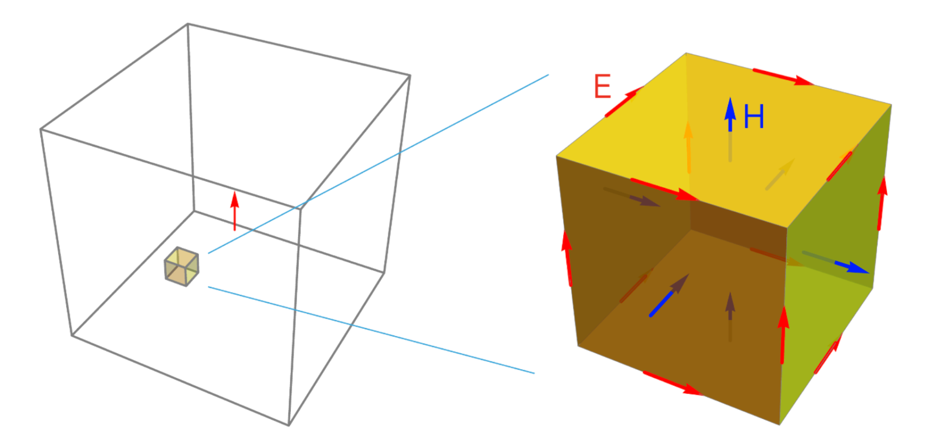
The first step of FDTD is discretizing the spatial and temporal dimensions on a regular, rectangular grid. In this formalism, the derivative operations in Maxwell’s equations may be approximated using “finite differences”. The FDTD algorithm then solves E(t) and H(t) one after another starting from t=0 and terminating when a final condition is met, for example when there are very little fields present in the system.
FDTD 101 White PaperModel a Photonic Device in FDTD
First, Specify the global simulation parameters, such as the size, discretization characteristics, and boundary conditions. These parameters define the context of the device and the discretization can be used as a knob to balance accuracy with speed.
Next, Specify all of the geometries and material properties of the structures within the domain. Afterwards, define the excitation that injects electromagnetic energy into this system. This can be done by directly specifying a current source, such as a point dipole, or a desired field pattern, such as a plane wave, from which a current source distribution can be defined.
Finally, Define the quantities of interest to be measured from the simulation. For example, measuring the time dynamics of a field component at a point within the simulation domain or the flux through a plane. Defining these “monitors” up front means that less information will need to be stored and many of these quantities can be computed during the run, saving time.
Useful References
Tidy3D is Flexcompute’s python-based FDTD solver, which makes it simple to define and run FDTD simulations.
EMPossible’s course on FDTD is very useful in leaning more about the implementation of FDTD
If your simulation diverges, follow this article and perform thorough troubleshooting.
Taflove FDTD is the main reference for the definitive guide to the method and all of the details.
“Inverse design” is a technique where one can use computational methods to automate the process of designing photonic devices. Master the art of simulation with our cutting-edge lectures
Discover simulation excellence! Find inspiration in our showcase of simulations.

