Authors: Gaurav Desai, Dr. Judson Ryckman, Clemson University
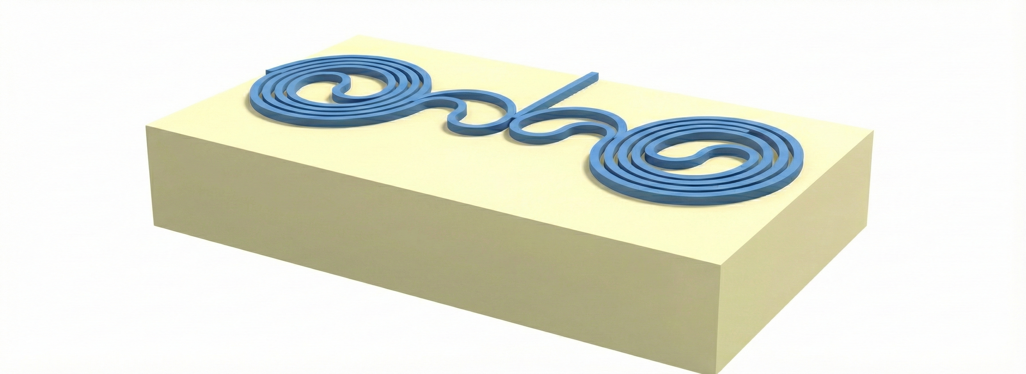
This script simulates a compact spiral resonator. The geometry is predefined via a layout (GDS import), layout_0. To emulate fabrication-induced symmetry breaking between the left and right spirals, the right spiral is intentionally modified to have an average width of 498 nm, while the left spiral retains an average width of 500 nm.
This illustrative simulation is performed in 2D by approximating the 3D problem using the effective index method (220 nm thick SOI at 1550 nm).
We perform an FDTD simulation to obtain a transmission spectrum indicative of the device’s resonant properties. Optionally, we can visualize the electric field to reveal how the resonances are localized.
import tidy3d as td
import numpy as np
import tidy3d.web as web
import matplotlib.pyplot as plt
import gdstk
Simulation Setup.
SiO2 = td.Medium(
    name="SiO2",
    permittivity=2.0736,
)

Silicon = td.Medium(
    name="Silicon",
    # Simplified 1D effective index approximation for a 220 nm SOI slab at 1550 nm (TE)
    permittivity=8.0656,
)

modesource_0 = td.ModeSource(
    name="modesource_0",
    center=[168.07, -30, 0],
    size=[5, 0, 5],
    source_time=td.GaussianPulse(
        freq0=193615962458333.3,
        fwidth=7000000000000,
    ),
    direction="-",
    mode_spec=td.ModeSpec(
        target_neff=2.84,
        precision="single",
        group_index_step=True,
        sort_spec={
            "filter_key": "TE_fraction",
            "filter_reference": 0.5,
            "filter_order": "over",
            "sort_order": "ascending",
            "track_freq": "central",
        },
    ),
)

fluxmonitor_0 = td.FluxMonitor(
    name="fluxmonitor_0",
    center=[168.07, -80, 0],
    size=[10, 0, 10],
    # Wavelength range from 1.5 µm to 1.6 µm
    freqs=td.C_0 / np.linspace(1.5, 1.6, 5001),
)

fieldmonitor_xy = td.FieldMonitor(
    name="fieldmonitor_xy",
    center=[168.07, -54, 0.25],
    size=[112, 55, 0],
    # Narrow wavelength range around resonance; can rerun at exact frequencies if needed
    freqs=td.C_0 / np.linspace(1.54925, 1.54975, 5),
)
15:41:06 -03 WARNING: A large number (5001) of frequencies detected in monitor
             'fluxmonitor_0'. This can lead to solver slow-down and increased
             cost. Consider decreasing the number of frequencies in the monitor.
             This may become a hard limit in future Tidy3D versions.
Load GDS layout.
gds_path = "misc/CompactDualSpiral.gds"

# Load the GDSII library from file
lib_loaded = gdstk.read_gds(gds_path)

# Create a dictionary mapping cell names to cell objects
all_cells = {c.name: c for c in lib_loaded.cells}
cell = all_cells["MAIN"]

# Convert the selected GDS cell into a Tidy3D geometry
geometry = td.Geometry.from_gds(
    cell,
    gds_layer=0,
    slab_bounds=(0, 0.5),
    axis=2,
)

# Create a structure from the imported geometry
layout_0 = td.Structure(
    geometry=geometry,
    name="layout_0",
    medium=Silicon,
)
First, we visualize the imported layout geometry.
ax1 = layout_0.plot(z=0.0)
plt.show()
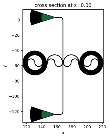
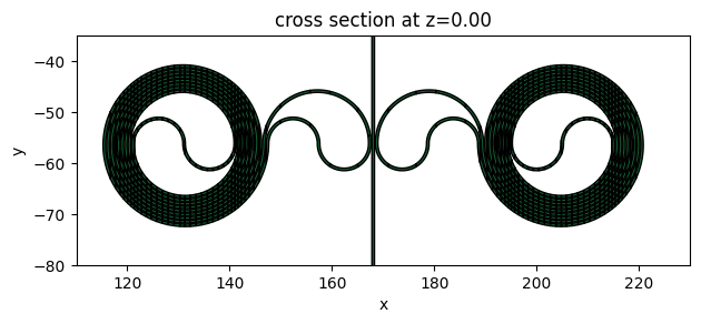
Our simulation will be 2D and will not include the grating couplers in the layout. Instead, we focus on the spiral resonator region, as shown below:
ax1 = layout_0.plot(z=0.0)
ax1.set_ylim(-80, -35)
ax1.set_xlim(110, 230)
plt.show()
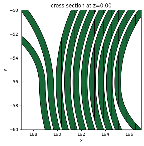
Here is a zoomed-in view of the spiral, showing the ~200 nm gaps.
ax1 = layout_0.plot(z=0.0)
ax1.set_ylim(-60, -50)
ax1.set_xlim(187, 197)
plt.show()
Next, we build and run the simulation. Optionally, you can comment out the web.run command and instead load a previously completed task in the next cell.
sim = td.Simulation(
    center=[166.625, -56, 0.25],
    size=[118, 65, 0],
    boundary_spec=td.BoundarySpec(
        x=td.Boundary(
            plus=td.PML(
                parameters=td.PMLParams(
                    kappa_min=1, kappa_max=3, alpha_order=1, alpha_max=0
                )
            ),
            minus=td.PML(
                parameters=td.PMLParams(
                    kappa_min=1, kappa_max=3, alpha_order=1, alpha_max=0
                )
            ),
        ),
        y=td.Boundary(
            plus=td.PML(
                parameters=td.PMLParams(
                    kappa_min=1, kappa_max=3, alpha_order=1, alpha_max=0
                )
            ),
            minus=td.PML(
                parameters=td.PMLParams(
                    kappa_min=1, kappa_max=3, alpha_order=1, alpha_max=0
                )
            ),
        ),
        z=td.Boundary(
            plus=td.Periodic(),
            minus=td.Periodic(),
        ),
    ),
    grid_spec=td.GridSpec(
        grid_x=td.AutoGrid(min_steps_per_wvl=15),
        grid_y=td.AutoGrid(min_steps_per_wvl=15),
        grid_z=td.AutoGrid(min_steps_per_wvl=15),
        wavelength=1.55,
    ),
    version="2.10.1",
    shutoff=1e-6,
    run_time=8.2e-10,
    medium=SiO2,
    sources=[modesource_0],
    monitors=[fluxmonitor_0, fieldmonitor_xy],
    structures=[layout_0],
)
# Comment out this line to skip running the simulation
sim_data = web.run(
    sim,
    task_name="SpiralResonator_asymm_FDTD",
    path="./data/sim_data.hdf5",
)
15:41:08 -03 WARNING: Simulation has 9.65e+06 time steps. The 'run_time' may be
             unnecessarily large, unless there are very long-lived resonances.
15:41:19 -03 Created task 'SpiralResonator_asymm_FDTD' with resource_id
             'fdve-89b4b497-58bf-451d-b59b-59bb4234fe6b' and task_type 'FDTD'.
             View task using web UI at
             'https://tidy3d.simulation.cloud/workbench?taskId=fdve-89b4b497-58b
             f-451d-b59b-59bb4234fe6b'.
Task folder: 'default'.
Output()
15:41:44 -03 Estimated FlexCredit cost: 16.796. Minimum cost depends on task
             execution details. Use 'web.real_cost(task_id)' to get the billed
             FlexCredit cost after a simulation run.
15:41:46 -03 status = queued
             To cancel the simulation, use 'web.abort(task_id)' or
             'web.delete(task_id)' or abort/delete the task in the web UI.
             Terminating the Python script will not stop the job running on the
             cloud.
Output()
15:41:56 -03 status = preprocess
15:42:10 -03 starting up solver
15:42:13 -03 running solver
Output()
15:49:43 -03 WARNING: No connection: Retrying for 180 seconds.
16:02:54 -03 early shutoff detected at 0%, exiting.
status = queued
Output()
16:03:15 -03 status = preprocess
16:03:20 -03 status = running
16:40:11 -03 WARNING: No connection: Retrying for 180 seconds.
16:51:57 -03 status = postprocess
16:52:25 -03 status = success
16:52:27 -03 View simulation result at
             'https://tidy3d.simulation.cloud/workbench?taskId=fdve-89b4b497-58b
             f-451d-b59b-59bb4234fe6b'.
Output()
16:53:27 -03 Loading simulation from data/sim_data.hdf5
16:53:28 -03 WARNING: A large number (5001) of frequencies detected in monitor
             'fluxmonitor_0'. This can lead to solver slow-down and increased
             cost. Consider decreasing the number of frequencies in the monitor.
             This may become a hard limit in future Tidy3D versions.
             WARNING: A large number (5001) of frequencies detected in monitor
             'fluxmonitor_0'. This can lead to solver slow-down and increased
             cost. Consider decreasing the number of frequencies in the monitor.
             This may become a hard limit in future Tidy3D versions.
             WARNING: Simulation final field decay value of 2.07e-06 is greater
             than the simulation shutoff threshold of 1e-06. Consider running
             the simulation again with a larger 'run_time' duration for more
             accurate results.
             WARNING: Warning messages were found in the solver log. For more
             information, check 'SimulationData.log' or use
             'web.download_log(task_id)'.
Post-Processing
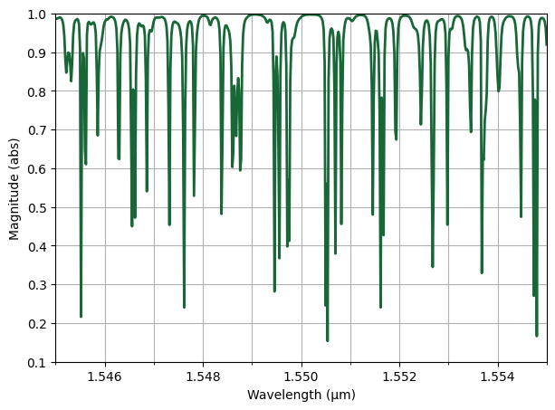
Next, we load and plot the transmission spectrum. Here, we observe irregularly spaced resonances indicative of the standing wave modes of each spiral resonator. There are up to four visibly distinct modes per FSR, corresponding to the two standing wave modes (symmetric and antisymmetric) localized in each spiral.
import matplotlib.pyplot as plt
import matplotlib.ticker as mticker

md = sim_data["fluxmonitor_0"]

# Extract flux data
flux = np.asarray(md.flux).squeeze()

# Compute magnitude of the flux
flux_abs = np.abs(flux)

# Extract frequency coordinates from the FluxData object
# (Works even if monitor.freqs is nested or tuple-based)
freqs = np.asarray(md.flux.coords["f"]).squeeze()
wl_um = td.C_0 / freqs  # Convert frequency to wavelength in microns

plt.figure(figsize=(7, 5))
plt.plot(wl_um, flux_abs, linewidth=2)

ax = plt.gca()

# Configure x-axis (wavelength)
ax.set_xlim(1.545, 1.555)
ax.xaxis.set_major_locator(mticker.MultipleLocator(0.002))
ax.xaxis.set_minor_locator(mticker.MultipleLocator(0.001))

# Configure y-axis (flux magnitude)
ax.set_ylim(0.1, 1.0)
ax.yaxis.set_major_locator(mticker.MultipleLocator(0.1))

plt.xlabel("Wavelength (µm)")
plt.ylabel("Magnitude (abs)")

ax.grid(True, which="both")
plt.show()
             WARNING: A large number (5001) of frequencies detected in monitor
             'fluxmonitor_0'. This can lead to solver slow-down and increased
             cost. Consider decreasing the number of frequencies in the monitor.
             This may become a hard limit in future Tidy3D versions.
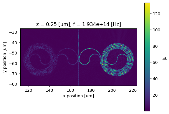
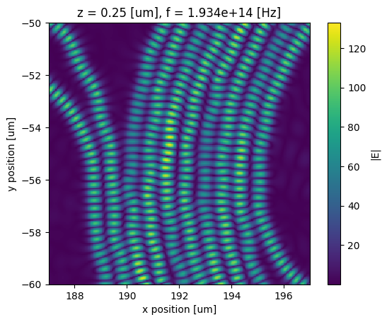
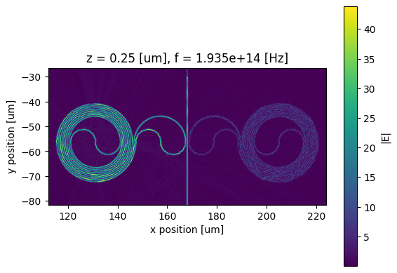
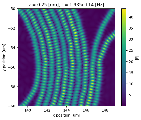
Lastly, we visualize the resonant E-field and observe the standing wave resonances. In the example below, we select two resonant frequencies from the spectrum and plot the corresponding field distributions.
# Optional: Visualize resonant E-field (e.g., localization in the left spiral)
s = sim_data._get_scalar_field(
    field_monitor_name="fieldmonitor_xy",
    field_name="E",
    val="abs",
)
plot_data = s.sel(z=0.25).sel(f=193476900935785.72)

# Plot the selected field distribution
if plot_data.size == 1:
    print(plot_data)
else:
    fig, ax = plt.subplots()
    plot_data.plot(x="x", y="y", ax=ax)
    ax.set_aspect("equal")

    fig, ax2 = plt.subplots()
    plot_data.plot(x="x", y="y", ax=ax2)
    ax2.set_ylim(-60, -50)
    ax2.set_xlim(139, 149)
    ax2.set_aspect("equal")
plt.show()
# Optional: Visualize resonant E-field (e.g., localization in the right spiral)
s = sim_data._get_scalar_field(
    field_monitor_name="fieldmonitor_xy",
    field_name="E",
    val="abs",
)
plot_data = s.sel(z=0.25).sel(f=193445689949991.94)

# Plot the selected field distribution
if plot_data.size == 1:
    print(plot_data)
else:
    fig, ax = plt.subplots()
    plot_data.plot(x="x", y="y", ax=ax)
    ax.set_aspect("equal")

    fig, ax2 = plt.subplots()
    plot_data.plot(x="x", y="y", ax=ax2)
    ax2.set_ylim(-60, -50)
    ax2.set_xlim(187, 197)
    ax2.set_aspect("equal")
plt.show()