Author: Federica Marinelli, Northeastern University
In this notebook, we use Tidy3D to model and analyze a compact broadband optical absorber designed for mid-infrared superconducting photon detectors.
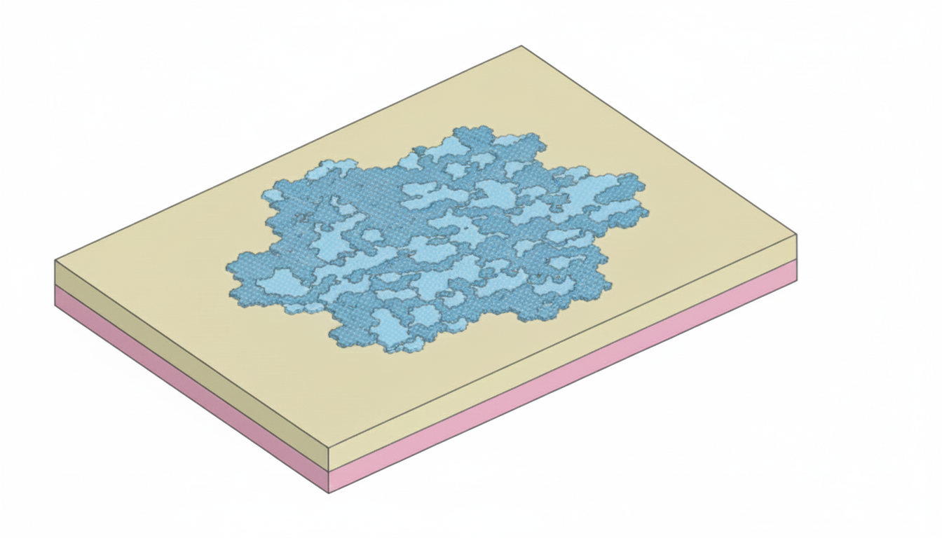
The structure is based on a fractal-inspired metallic pattern, which enables strong light trapping and broadband absorption within a subwavelength footprint. The self-similar geometry supports multiple resonant modes across the mid-IR, enhancing absorption efficiency while maintaining compactness—an important requirement for integration with superconducting detector platforms.
The simulation involves a Gaussian beam incident on the structure, considering both TE and TM polarizations.
import tidy3d as td
import tidy3d.web as web

import matplotlib.pyplot as plt
from tidy3d.plugins.dispersion import FastDispersionFitter, AdvancedFastFitterParam

import pandas as pd
import numpy as np
Simulation Setup
First, we will import the geometry from the GDS file. The GDS and other files can be found in our Github page.
import gdstk

fractal_t = 0.020

lib_loaded = gdstk.read_gds("misc/gosper_fractal_geometry.gds")
cell = lib_loaded.top_level()[0]

fractal_geo = td.Geometry.from_gds(
    cell,
    gds_layer=0,
    gds_dtype=0,
    axis=2,
    slab_bounds=(-fractal_t / 2, fractal_t / 2),
    reference_plane="bottom",
)
Defining global parameters.
# parameters wavelength and material
wl_c = 1.55  # central wavelength.
wl_n = 1001  # number of wavelength points to compute the output data.
freq0 = td.C_0 / wl_c  # central frequency.
freq_bw = 150e12
freqs = np.linspace(freq0 - freq_bw, freq0 + freq_bw, wl_n)
lambdas = td.C_0 / freqs

mat_dielectric = td.material_library["SiO2"]["Horiba"]
mat_air = td.Medium(permittivity=1.00)
Fitting media
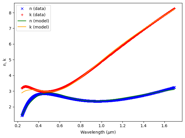
Next, we will create Medium objects from experimental permittivity data. To do so, we will use the AdvancedFastFitterParam object.
file = "misc/Rakic_LD_wl_n_k.csv"

fitter = FastDispersionFitter.from_file(file, skiprows=2, delimiter=",")


advanced_param = AdvancedFastFitterParam(weights=(1, 1))
gold, rms_error = fitter.fit(
    max_num_poles=3, advanced_param=advanced_param, tolerance_rms=2e-2
)
fitter.plot(gold)
plt.show()
Output()
17:18:04 E. South America Standard Time WARNING: Unable to fit with weighted RMS
                                        error under 'tolerance_rms' of 0.02
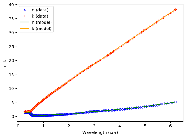
file = "misc/Nb.csv"

fitter = FastDispersionFitter.from_file(file, skiprows=2, delimiter=",")

plt.show()

advanced_param = AdvancedFastFitterParam(
    weights=(1, 1)
)
mat_Nb, rms_error = fitter.fit(
    max_num_poles=7, advanced_param=advanced_param, tolerance_rms=2e-2
)
fitter.plot(mat_Nb)
plt.show()
Output()
17:21:53 E. South America Standard Time WARNING: Unable to fit with weighted RMS
                                        error under 'tolerance_rms' of 0.02
Defining the substrate and medium.
dielectric_t = 1.35  # µm

# simulation domain size
Lx, Ly, Lz = 20, 20, wl_c * 2.5
sim_size = [Lx, Ly, Lz]

# construct the gold substrate
substrate = td.Structure(
    geometry=td.Box(
        center=[0, 0, -wl_c / 2 - dielectric_t / 2], size=[td.inf, td.inf, wl_c]
    ),
    medium=gold,
)

# construct the dielectric substrate

dielectric = td.Structure(
    geometry=td.Box(center=[0, 0, 0], size=[td.inf, td.inf, dielectric_t]),
    medium=mat_dielectric,
)
Now we define a GaussianBeam beam source and two FluxMonitors to calculate transmission and reflection.
spot_size = 5.0  # um, spot size of the Gaussian beam
# add a Gaussian beam source
gaussian_beam = td.GaussianBeam(
    source_time=td.GaussianPulse(freq0=freq0, fwidth=freq_bw),
    size=(td.inf, td.inf, 0),
    center=(0, 0, 0.4 * Lz),
    direction="-",
    pol_angle=0,
    waist_radius=spot_size / 2,
)


# add a flux monitor to detect transmission
monitor_t = td.FluxMonitor(
    center=[0, 0, -0.4 * Lz],
    size=[td.inf, td.inf, 0],
    freqs=freqs,
    name="T",
)

# add a flux monitor to detect reflection
monitor_r = td.FluxMonitor(
    center=[0, 0, 0.5 * Lz],
    size=[td.inf, td.inf, 0],
    freqs=freqs,
    name="R",
)
Defining the Simulation object.
run_time = 1e-12  # simulation run time

fractal = td.Structure(geometry=fractal_geo, medium=mat_Nb)


sim_nb = td.Simulation(
    center=(0, 0, dielectric_t / 8),
    size=sim_size,
    medium=mat_air,
    grid_spec=td.GridSpec(
        grid_x=td.AutoGrid(min_steps_per_wvl=6),
        grid_y=td.AutoGrid(min_steps_per_wvl=6),
        grid_z=td.AutoGrid(min_steps_per_wvl=50),
    ),
    structures=[substrate, dielectric, fractal],
    sources=[gaussian_beam],
    monitors=[monitor_t, monitor_r],
    run_time=run_time,
    boundary_spec=td.BoundarySpec(
        x=td.Boundary.pml(num_layers=20),
        y=td.Boundary.pml(num_layers=20),
        z=td.Boundary.pml(num_layers=20),
    ),
    symmetry=(0, 0, 0),
)
17:21:54 E. South America Standard Time WARNING: The medium associated with
                                        'SiO2_Horiba' (simulation.mediums[2])
                                        has a frequency range: (1.6926e14,
                                        12.0899e14) (Hz) that does not fully
                                        cover the frequencies contained in 'T'
                                        (simulation.monitors[0]).This can cause
                                        inaccuracies in the recorded results.
WARNING: Suppressed 1 WARNING message.
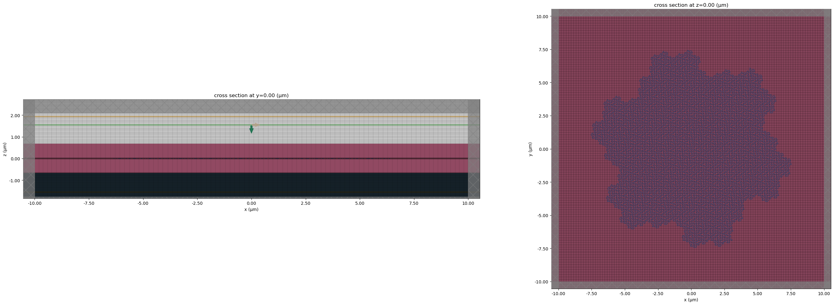
Visualizing the setup.
fig, (ax1, ax2) = plt.subplots(1, 2, tight_layout=True, figsize=(30, 10))
ax1 = sim_nb.plot(y=0, ax=ax1)
ax1 = sim_nb.plot_grid(y=0, ax=ax1)

ax2 = sim_nb.plot(z=0, ax=ax2)
ax2 = sim_nb.plot_grid(z=0, ax=ax2)

plt.show()
Running for TM mode
sim_data_nb = web.run(sim_nb, task_name="fractal_nb", path="data/simulation.hdf5")
17:22:01 E. South America Standard Time Created task 'fractal_nb' with task_id
                                        'fdve-c5232a2f-78d6-4987-9ac0-39b2092bb1
                                        ba' and task_type 'FDTD'.
                                        View task using web UI at
                                        'https://tidy3d.simulation.cloud/workben
                                        ch?taskId=fdve-c5232a2f-78d6-4987-9ac0-3
                                        9b2092bb1ba'.
Task folder: 'default'.
Output()
17:23:01 E. South America Standard Time Maximum FlexCredit cost: 19.172. Minimum
                                        cost depends on task execution details.
                                        Use 'web.real_cost(task_id)' to get the
                                        billed FlexCredit cost after a
                                        simulation run.
17:23:22 E. South America Standard Time status = queued
                                        To cancel the simulation, use
                                        'web.abort(task_id)' or
                                        'web.delete(task_id)' or abort/delete
                                        the task in the web UI. Terminating the
                                        Python script will not stop the job
                                        running on the cloud.
Output()
17:24:00 E. South America Standard Time status = preprocess
17:24:21 E. South America Standard Time starting up solver
running solver
Output()
17:25:36 E. South America Standard Time early shutoff detected at 12%, exiting.
status = postprocess
Output()
17:25:38 E. South America Standard Time status = success
17:25:40 E. South America Standard Time View simulation result at
                                        'https://tidy3d.simulation.cloud/workben
                                        ch?taskId=fdve-c5232a2f-78d6-4987-9ac0-3
                                        9b2092bb1ba'.
Output()
17:25:45 E. South America Standard Time loading simulation from
                                        data/simulation.hdf5
17:25:59 E. South America Standard Time WARNING: The medium associated with
                                        'SiO2_Horiba' (simulation.mediums[2])
                                        has a frequency range: (1.6926e14,
                                        12.0899e14) (Hz) that does not fully
                                        cover the frequencies contained in 'T'
                                        (simulation.monitors[0]).This can cause
                                        inaccuracies in the recorded results.
WARNING: Suppressed 1 WARNING message.
                                        WARNING: Warning messages were found in
                                        the solver log. For more information,
                                        check 'SimulationData.log' or use
                                        'web.download_log(task_id)'.
Post-process
First, we look at the monitors to obtain reflection and transmission data, and calculate the losses using R + T + A = 1.
plt.figure(figsize=(8, 5))
R_nb = sim_data_nb["R"].flux
T_nb = -sim_data_nb["T"].flux
A_nb = 1 - R_nb - T_nb
plt.plot(lambdas, R_nb, lambdas, T_nb, lambdas, A_nb)
plt.xlabel("Wavelength (μm)")

plt.legend(("Reflection", "Transmission", "Absorption"))
plt.show()

data = pd.DataFrame({"Wavelength_um": lambdas, "R": R_nb, "T": T_nb, "A": A_nb})

data.to_csv("sim_data_nb.csv", index=False)
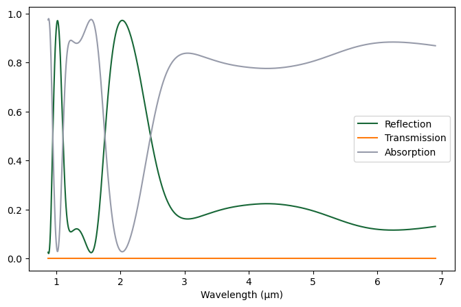
mask = lambdas > 3

A_nb_filtered = A_nb[mask]

mean_A_nb = np.mean(A_nb_filtered)

print(f"{mean_A_nb:.4f}")
0.8181
Running for TE mode
Next, we can run the same setup changing the source polarization.
gaussian_beam_TE = td.GaussianBeam(
    source_time=td.GaussianPulse(freq0=freq0, fwidth=freq_bw),
    size=(td.inf, td.inf, 0),
    center=(0, 0, 0.4 * Lz),
    direction="-",
    pol_angle=np.pi / 2,  # Rotate the polarization angle by 90 degrees
    waist_radius=spot_size / 2,
)

sim_TE = sim_nb.updated_copy(sources=[gaussian_beam_TE])
17:26:01 E. South America Standard Time WARNING: The medium associated with
                                        'SiO2_Horiba' (simulation.mediums[2])
                                        has a frequency range: (1.6926e14,
                                        12.0899e14) (Hz) that does not fully
                                        cover the frequencies contained in 'T'
                                        (simulation.monitors[0]).This can cause
                                        inaccuracies in the recorded results.
WARNING: Suppressed 1 WARNING message.
sim_data_nb_TE = web.run(sim_TE, task_name="fractal_nb_TE", path="data/simulation.hdf5")
                                        Created task 'fractal_nb_TE' with
                                        task_id
                                        'fdve-a1cb5200-32be-477c-b23b-4fa9185e7b
                                        7b' and task_type 'FDTD'.
                                        View task using web UI at
                                        'https://tidy3d.simulation.cloud/workben
                                        ch?taskId=fdve-a1cb5200-32be-477c-b23b-4
                                        fa9185e7b7b'.
Task folder: 'default'.
Output()
17:27:05 E. South America Standard Time Maximum FlexCredit cost: 19.172. Minimum
                                        cost depends on task execution details.
                                        Use 'web.real_cost(task_id)' to get the
                                        billed FlexCredit cost after a
                                        simulation run.
17:27:06 E. South America Standard Time status = queued
                                        To cancel the simulation, use
                                        'web.abort(task_id)' or
                                        'web.delete(task_id)' or abort/delete
                                        the task in the web UI. Terminating the
                                        Python script will not stop the job
                                        running on the cloud.
Output()
17:27:24 E. South America Standard Time status = preprocess
17:27:45 E. South America Standard Time starting up solver
running solver
Output()
17:29:01 E. South America Standard Time early shutoff detected at 12%, exiting.
status = postprocess
Output()
17:29:04 E. South America Standard Time status = success
17:29:06 E. South America Standard Time View simulation result at
                                        'https://tidy3d.simulation.cloud/workben
                                        ch?taskId=fdve-a1cb5200-32be-477c-b23b-4
                                        fa9185e7b7b'.
Output()
17:29:10 E. South America Standard Time loading simulation from
                                        data/simulation.hdf5
17:29:23 E. South America Standard Time WARNING: The medium associated with
                                        'SiO2_Horiba' (simulation.mediums[2])
                                        has a frequency range: (1.6926e14,
                                        12.0899e14) (Hz) that does not fully
                                        cover the frequencies contained in 'T'
                                        (simulation.monitors[0]).This can cause
                                        inaccuracies in the recorded results.
WARNING: Suppressed 1 WARNING message.
                                        WARNING: Warning messages were found in
                                        the solver log. For more information,
                                        check 'SimulationData.log' or use
                                        'web.download_log(task_id)'.
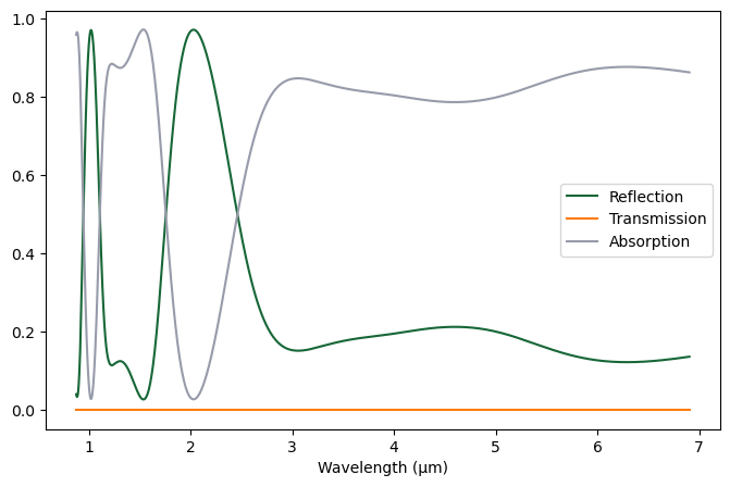
TE post-process
plt.figure(figsize=(8, 5))
R_nb_TE = sim_data_nb_TE["R"].flux
T_nb_TE = -sim_data_nb_TE["T"].flux
A_nb_TE = 1 - R_nb_TE - T_nb_TE
plt.plot(lambdas, R_nb_TE, lambdas, T_nb_TE, lambdas, A_nb_TE)
plt.xlabel("Wavelength (μm)")


plt.legend(("Reflection", "Transmission", "Absorption"))
plt.show()

data = pd.DataFrame(
    {"Wavelength_um": lambdas, "R": R_nb_TE, "T": T_nb_TE, "A": A_nb_TE}
)

data.to_csv("sim_data_nb_TE.csv", index=False)
Comparing TE and TM
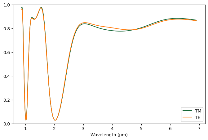
Finally, we can plot both TE and TM absorption together, calculate the correlation, and confirm that the absorption is almost invariant with polarization.
plt.figure(figsize=(8, 5))
plt.plot(lambdas, A_nb, lambdas, A_nb_TE)
plt.xlabel("Wavelength (μm)")
plt.ylim(0, 1)
plt.legend(("TM", "TE"))
plt.show()
# Select the wavelength range 3–7 µm
mask = (lambdas >= 3) & (lambdas <= 7)

# Compute mean absolute difference
mad = np.mean(np.abs(A_nb[mask] - A_nb_TE[mask]))
print(f"Mean absolute difference (3–7 µm): {mad:.4f}")

mean_absorption = np.mean((A_nb[mask] + A_nb_TE[mask]) / 2)
rel_diff = mad / mean_absorption * 100
print(f"Relative difference (3–7 µm): {rel_diff:.2f}%")

r = np.corrcoef(A_nb[mask], A_nb_TE[mask])[0, 1]
print(f"Correlation coefficient (3–7 µm): {r:.3f}")
Mean absolute difference (3–7 µm): 0.0126
Relative difference (3–7 µm): 1.54%
Correlation coefficient (3–7 µm): 0.951