Author: Dr. Chenchen Wang, University of Wisconsin–Madison
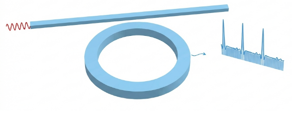
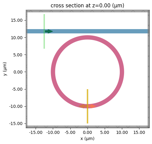
We use finite-difference time-domain (FDTD) simulations to study dissipative Kerr soliton formation in a Kerr nonlinear ring resonator. To efficiently access the soliton regime, we adopt a soft-seeding approach: a short pump pulse is applied as an initial condition and is followed by continuous-wave (CW) pumping. Using this method, we obtain stable Kerr solitons and characterize their temporal waveforms and optical spectra. By tuning the pump conditions, we further observe breathing solitons, demonstrating the transition from stationary to periodically oscillating soliton dynamics within the same FDTD framework. For more details, see https://www.flexcompute.com/tidy3d/community/notebooks/2DKerr/.
The total simulation takes around one hour and costs around 7 credits.
import matplotlib.pyplot as plt
import numpy as np
import tidy3d as td
import tidy3d.web as web
from tidy3d.plugins.mode import ModeSolver
Simulation Setup
# ---------------------------
# Parameter Definitions
# ---------------------------
# Geometrical parameters
wg_width = 1.25
couple_width = 0.5
ring_radius = 10
ring_wg_width = wg_width
wg_spacing = 2.5
buffer = 5.0

# Simulation dimensions
x_span = 2 * wg_spacing + 2 * ring_radius + 2 * buffer
y_span = 2 * ring_radius + ring_wg_width + wg_width + couple_width + 2 * buffer
sim_center_y = (couple_width + wg_width) / 2
wg_insert_x = ring_radius + wg_spacing
wg_center_y = ring_radius + ring_wg_width / 2.0 + couple_width + wg_width / 2.0

# Wavelength and frequency parameters
freq0 = 195.835e12
amp = 18
run_time = 400e-12
min_steps_per_wvl = 30
fwidth = 44.9689e12

# ---------------------------
# Medium Definitions
# ---------------------------
n_bg = 1.0
n_solid = 1.5
background = td.Medium(permittivity=n_bg**2)
solid = td.Medium(permittivity=n_solid**2)

n_kerr_2 = 2.0e-8
kerr_chi3 = 4 * (n_solid**2) * td.constants.EPSILON_0 * td.constants.C_0 * n_kerr_2 / 3
chi3_model = td.NonlinearSpec(
    models=[td.NonlinearSusceptibility(chi3=kerr_chi3)], num_iters=10
)
kerr_solid = td.Medium(permittivity=n_solid**2, nonlinear_spec=chi3_model)
# ---------------------------
# Structure and Simulation Region Definitions
# ---------------------------
# Define structure
waveguide = td.Structure(
    geometry=td.Box(
        center=[0, wg_center_y, 0],
        size=[td.inf, wg_width, td.inf],
    ),
    medium=solid,
    name="waveguide",
)
# Ring Structure
outer = td.Cylinder(
    center=[0, 0, 0],
    axis=2,
    radius=ring_radius + ring_wg_width / 2.0,
    length=td.inf,
)
inner = td.Cylinder(
    center=[0, 0, 0],
    axis=2,
    radius=ring_radius - ring_wg_width / 2.0,
    length=td.inf,
)
ring = td.Structure(
    geometry=outer - inner,
    medium=kerr_solid,
    name="outer_ring",
)
# Define mode plane and ring mode plane
mode_plane = td.Box(center=[-wg_insert_x, wg_center_y, 0], size=[0, 10, td.inf])
ring_mode_plane = td.Box(center=[0, -ring_radius, 0], size=[0, 10, td.inf])
# ---------------------------
# Mode Solver Setup
# ---------------------------
sim_modesolver = td.Simulation(
    center=[0, sim_center_y, 0],
    size=[x_span, y_span, 0],
    grid_spec=td.GridSpec.auto(
        min_steps_per_wvl=min_steps_per_wvl, wavelength=td.C_0 / freq0
    ),
    structures=[waveguide],
    run_time=1e-12,
    boundary_spec=td.BoundarySpec.all_sides(boundary=td.Periodic()),
    medium=background,
)

mode_spec = td.ModeSpec(num_modes=2)
mode_solver = ModeSolver(
    simulation=sim_modesolver, plane=mode_plane, mode_spec=mode_spec, freqs=[freq0]
)
mode_data = web.run(mode_solver, "mode_solver_kerr")
13:55:53 -03 Created task 'mode_solver_kerr' with task_id
             'mo-da2003b6-dca1-4c93-97f5-0e3a2d2aeaa1' and task_type
             'MODE_SOLVER'.
             View task using web UI at
             'https://tidy3d.simulation.cloud/workbench?taskId=mo-da2003b6-dca1-
             4c93-97f5-0e3a2d2aeaa1'.
Task folder: 'default'.
Output()
13:55:56 -03 Maximum FlexCredit cost: 0.004. Minimum cost depends on task
             execution details. Use 'web.real_cost(task_id)' to get the billed
             FlexCredit cost after a simulation run.
13:55:58 -03 status = queued
             To cancel the simulation, use 'web.abort(task_id)' or
             'web.delete(task_id)' or abort/delete the task in the web UI.
             Terminating the Python script will not stop the job running on the
             cloud.
Output()
13:56:03 -03 starting up solver
running solver
13:56:05 -03 status = success
             View simulation result at
             'https://tidy3d.simulation.cloud/workbench?taskId=mo-da2003b6-dca1-
             4c93-97f5-0e3a2d2aeaa1'.
Output()
13:56:07 -03 loading simulation from simulation_data.hdf5
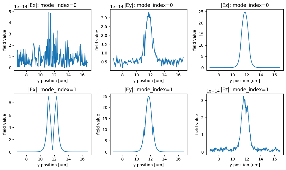
f, ((ax1, ax2, ax3), (ax4, ax5, ax6)) = plt.subplots(
    2, 3, tight_layout=True, figsize=(10, 6)
)

mode_data.Ex.sel(mode_index=0, f=freq0).abs.plot(ax=ax1)
mode_data.Ey.sel(mode_index=0, f=freq0).abs.plot(ax=ax2)
mode_data.Ez.sel(mode_index=0, f=freq0).abs.plot(ax=ax3)
mode_data.Ex.sel(mode_index=1, f=freq0).abs.plot(ax=ax4)
mode_data.Ey.sel(mode_index=1, f=freq0).abs.plot(ax=ax5)
mode_data.Ez.sel(mode_index=1, f=freq0).abs.plot(ax=ax6)
ax1.set_title("|Ex|: mode_index=0")
ax2.set_title("|Ey|: mode_index=0")
ax3.set_title("|Ez|: mode_index=0")
ax4.set_title("|Ex|: mode_index=1")
ax5.set_title("|Ey|: mode_index=1")
ax6.set_title("|Ez|: mode_index=1")

mode_data.to_dataframe()

plt.show()
| wavelength | n eff | k eff | TE (Ey) fraction | wg TE fraction | wg TM fraction | mode area | ||
|---|---|---|---|---|---|---|---|---|
| f | mode_index | |||||||
| 1.958350e+14 | 0 | 1.530842 | 1.430577 | 0.0 | 2.183825e-30 | 1.000000 | 0.932933 | 1.167536 |
| 1 | 1.530842 | 1.406249 | 0.0 | 1.000000e+00 | 0.883778 | 1.000000 | 1.293469 |
# ---------------------------
# Monitor Settings
# ---------------------------
# Define measurement frequency range for the ring mode monitors
freq_beg = 150e12
freq_end = 241.6e12

freqs_measure = np.linspace(freq_beg, freq_end, 2001)
time_window = [390, 400]
apodization = td.ApodizationSpec(
    start=1e-12 * time_window[0], end=1e-12 * time_window[1], width=2e-14
)


ring_mode_monitor = td.ModeMonitor(
    size=ring_mode_plane.size,
    center=ring_mode_plane.center,
    freqs=freqs_measure,
    mode_spec=td.ModeSpec(num_modes=2),
    apodization=apodization,
    name="ring_mode",
)

ring_flux_monitor = td.FluxTimeMonitor(
    size=ring_mode_plane.size,
    center=ring_mode_plane.center,
    name="ring_flux",
)

mode_source = td.ModeSource(
    size=mode_plane.size,
    center=mode_plane.center,
    source_time=td.ContinuousWave(freq0=freq0, fwidth=fwidth, amplitude=amp),
    mode_spec=td.ModeSpec(num_modes=2),
    mode_index=1,
    direction="+",
    num_freqs=11,
)

pulse_source = td.ModeSource(
    size=ring_mode_plane.size,
    center=ring_mode_plane.center,
    source_time=td.GaussianPulse(amplitude=300, freq0=freq0, fwidth=fwidth),
    num_freqs=11,
    direction="-",
    mode_spec=td.ModeSpec(num_modes=2),
    mode_index=1,
)

# ---------------------------
# Overall Simulation Setup
# ---------------------------
sim = td.Simulation(
    normalize_index=None,
    center=[0, sim_center_y, 0],
    size=[x_span, y_span, 0],
    grid_spec=td.GridSpec.auto(
        min_steps_per_wvl=min_steps_per_wvl, wavelength=td.C_0 / freq0
    ),
    structures=[waveguide, ring],
    sources=[mode_source, pulse_source],
    monitors=[ring_mode_monitor, ring_flux_monitor],
    run_time=run_time,
    boundary_spec=td.BoundarySpec(
        x=td.Boundary.pml(), y=td.Boundary.pml(), z=td.Boundary.periodic()
    ),
    medium=background,
    shutoff=0,
)

sim.plot(z=0)
plt.show()
13:56:08 -03 WARNING: A large number (2001) of frequencies detected in monitor
             'ring_mode'. This can lead to solver slow-down and increased cost.
             Consider decreasing the number of frequencies in the monitor. This
             may become a hard limit in future Tidy3D versions.
             WARNING: The monitor 'interval' field was left as its default
             value, which will set it to 1 internally. A value of 1 means that
             the data will be sampled at every time step, which may potentially
             produce more data than desired, depending on the use case. To
             reduce data storage, one may downsample the data by setting
             'interval > 1' or by choosing alternative 'start' and 'stop' values
             for the time sampling. If you intended to use the highest
             resolution time sampling, you may suppress this warning by
             explicitly setting 'interval=1' in the monitor.
             WARNING: Using old versions of the shapely library (prior to v2.1)
             may cause plot errors.  This can be solved by upgrading to Python
             3.10 (or later) and reinstalling Tidy3d.
# ---------------------------
# Run Simulation Task
# ---------------------------
sim_data = web.run(
    sim,
    task_name="2DKerrSoliton",
    path="data/simulation_data.hdf5",
    verbose=True,
)
             WARNING: Simulation has 5.06e+06 time steps. The 'run_time' may be
             unnecessarily large, unless there are very long-lived resonances.
13:56:09 -03 Created task '2DKerrSoliton' with task_id
             'fdve-0f45fc3b-1da7-428b-951c-0683bceba02e' and task_type 'FDTD'.
             View task using web UI at
             'https://tidy3d.simulation.cloud/workbench?taskId=fdve-0f45fc3b-1da
             7-428b-951c-0683bceba02e'.
Task folder: 'default'.
Output()
13:56:11 -03 Maximum FlexCredit cost: 3.377. Minimum cost depends on task
             execution details. Use 'web.real_cost(task_id)' to get the billed
             FlexCredit cost after a simulation run.
13:56:13 -03 status = queued
             To cancel the simulation, use 'web.abort(task_id)' or
             'web.delete(task_id)' or abort/delete the task in the web UI.
             Terminating the Python script will not stop the job running on the
             cloud.
Output()
13:56:22 -03 status = preprocess
13:57:03 -03 starting up solver
running solver
Output()
14:36:21 -03 status = postprocess
Output()
14:36:26 -03 status = success
14:36:28 -03 View simulation result at
             'https://tidy3d.simulation.cloud/workbench?taskId=fdve-0f45fc3b-1da
             7-428b-951c-0683bceba02e'.
Output()
14:36:34 -03 loading simulation from data/simulation_data.hdf5
             WARNING: A large number (2001) of frequencies detected in monitor
             'ring_mode'. This can lead to solver slow-down and increased cost.
             Consider decreasing the number of frequencies in the monitor. This
             may become a hard limit in future Tidy3D versions.
             WARNING: Warning messages were found in the solver log. For more
             information, check 'SimulationData.log' or use
             'web.download_log(task_id)'.
Visualization Function
import matplotlib.pyplot as plt
import numpy as np
from scipy.signal import argrelextrema


# ----------------------------
# Small utilities (internal)
# ----------------------------
def _to_numpy(x):
    """Return a NumPy array from NumPy/xarray-like input."""
    return np.asarray(x.values) if hasattr(x, "values") else np.asarray(x)


def _get_time_axis(time_data, total_time=None):
    """
    Extract time coordinate from an xarray-like object if available.
    Otherwise, build a uniform time axis using `total_time`.
    """
    # Prefer xarray coords: time_data.coords['t'] or ['time']
    if hasattr(time_data, "coords"):
        for key in ("t", "time"):
            if key in time_data.coords:
                return np.asarray(time_data.coords[key].values)

    # Fallback: time_data.t (some objects expose this)
    if hasattr(time_data, "t"):
        try:
            return np.asarray(time_data.t.values)
        except Exception:
            pass

    # Last resort: uniform axis
    if total_time is None:
        raise ValueError(
            "No time coordinate found in `time_data`. Provide `total_time` (seconds) "
            "or pass an object containing time coords (e.g., time_data.coords['t'])."
        )
    y = _to_numpy(time_data)
    return np.linspace(0.0, total_time, len(y), endpoint=False)


# ----------------------------
# 1) Round-trip integrated flux
# ----------------------------
def plot_roundtrip_flux(
    flux_data, run_time=400, roundtrip_time=0.3310882353, line_color="b"
):
    """
    Integrate (sum) the flux within each round-trip window and plot versus time.

    Notes
    -----
    - Integration uses a simple summation over samples (same as original).
    - Time axis is built as uniform sampling over [0, run_time) (same as original).
    """
    y = _to_numpy(flux_data)

    n = len(y)
    t = np.linspace(0, run_time, n, endpoint=False)

    n_rt = int(run_time / roundtrip_time)

    rt_times = []
    rt_flux = []

    for i in range(n_rt):
        t0 = i * roundtrip_time
        t1 = (i + 1) * roundtrip_time
        tc = 0.5 * (t0 + t1)

        i0 = np.searchsorted(t, t0)
        i1 = np.searchsorted(t, t1)

        if i1 > i0:
            rt_times.append(tc)
            rt_flux.append(np.sum(y[i0:i1]))

    rt_times = np.asarray(rt_times)
    rt_flux = np.asarray(rt_flux)

    fig, ax = plt.subplots(figsize=(9, 3.3), dpi=100)
    ax.plot(rt_times, rt_flux, color=line_color, linewidth=1.5)

    ax.set_yticks([])
    ax.set_xlabel("Time (ps)", fontsize=12)
    ax.set_ylabel("Intracavity Energy (a.u.)", fontsize=12)

    plt.tight_layout()
    plt.show()


# ----------------------------
# 2) Frequency spectrum plot
# ----------------------------
def plot_frequency_spectrum(
    monitor_data,
    time_ps=395,
    mode_index=1,
    direction="-",
    ylim=(-320, -200),
    figsize=(9, 3.3),
    color="gray",
):
    """
    Plot a line spectrum (vlines) from monitor data at a given time label.

    Assumes
    -------
    monitor_data.amps.abs.sel(mode_index=..., direction=...) is available,
    and monitor_data.amps.f provides frequencies in Hz.
    """
    fig, ax = plt.subplots(figsize=figsize)

    amps = np.array(
        monitor_data.amps.abs.sel(mode_index=mode_index, direction=direction)
    )
    log_data = 20 * np.log10(amps)
    freqs_thz = np.array(monitor_data.amps.f) / 1e12

    ax.vlines(freqs_thz, ymin=ylim[0], ymax=log_data, color=color)
    ax.set_ylim(ylim)
    ax.set_title(f"Frequency Spectrum at {time_ps} ps")

    ax.set_yticklabels([])
    ax.set_ylabel("Power 20 dB / div")
    ax.set_xlabel("Frequency (THz)")

    plt.tight_layout()
    plt.show()


# ----------------------------
# 3) Local maxima in a time window
# ----------------------------
def plot_time_window_maxima(
    time_data,
    start_time,
    end_time,
    roundtrip_time=0.3310882353,
    min_height=None,
    min_distance=3,
    total_time=None,
    time_unit_for_plot="ps",
    ylim=(0, 1e5),
):
    """
    Plot raw time data in a window and overlay a curve through local maxima.

    Parameters
    ----------
    time_data : array-like or xarray-like
        Time series samples. If it contains time coordinates ('t' or 'time'), they are used.
        Otherwise provide `total_time` (seconds) to build a uniform axis.
    start_time, end_time : float
        Window bounds in seconds (same as original code behavior).
    min_height : float or None
        Optional threshold for maxima values.
    min_distance : int
        Neighborhood size (in points) for argrelextrema(order=...).
    time_unit_for_plot : {"s","ns","ps","fs"}
        Display unit for the time axis.
    ylim : tuple or None
        y-axis limits.
    """
    if end_time <= start_time:
        raise ValueError("end_time must be greater than start_time.")

    y = _to_numpy(time_data)
    t = _get_time_axis(time_data, total_time=total_time)

    i0 = int(np.searchsorted(t, start_time, side="left"))
    i1 = int(np.searchsorted(t, end_time, side="left"))
    i0 = max(0, min(i0, len(y)))
    i1 = max(0, min(i1, len(y)))

    y_win = y[i0:i1]
    t_win = t[i0:i1]

    max_idx = argrelextrema(y_win, np.greater, order=min_distance)[0]
    if min_height is not None and len(max_idx) > 0:
        max_idx = max_idx[y_win[max_idx] >= min_height]

    t_max = t_win[max_idx]
    y_max = y_win[max_idx]

    unit_scale = {"s": 1.0, "ns": 1e-9, "ps": 1e-12, "fs": 1e-15}
    if time_unit_for_plot not in unit_scale:
        raise ValueError("time_unit_for_plot must be one of: 's', 'ns', 'ps', 'fs'.")

    scale = unit_scale[time_unit_for_plot]
    t_win_disp = t_win / scale
    t_max_disp = t_max / scale

    start_disp = start_time / scale
    end_disp = end_time / scale
    _ = roundtrip_time / scale  # kept for parity; not used in plotting (same effect)

    plt.figure(figsize=(9, 3.3))
    plt.plot(
        t_win_disp,
        y_win,
        color="lightgray",
        alpha=1,
        linewidth=0.5,
        label="flux Data",
    )

    if len(t_max) > 1:
        # Keep the exact original behavior: spline only if > 5 maxima, else connect points.
        if len(t_max) > 5:
            from scipy.interpolate import make_interp_spline

            xnew = np.linspace(t_max_disp[0], t_max_disp[-1], 300)
            spl = make_interp_spline(t_max_disp, y_max, k=3)
            ynew = spl(xnew)
            plt.plot(xnew, ynew, alpha=0.7, linewidth=2, label="pulse envelope")
        else:
            plt.plot(t_max_disp, y_max, alpha=0.7, linewidth=2, label="pulse envelope")

    plt.title(
        f"Time window: {start_disp:.6g}{time_unit_for_plot} to {end_disp:.6g}{time_unit_for_plot}"
    )
    plt.xlabel(f"Time ({time_unit_for_plot})")
    plt.ylabel("Flux (a.u.)")
    plt.grid(True, alpha=0.3)
    plt.legend()
    plt.yticks([])

    if ylim is not None:
        plt.ylim(*ylim)

    plt.tight_layout()
    plt.show()
Soliton
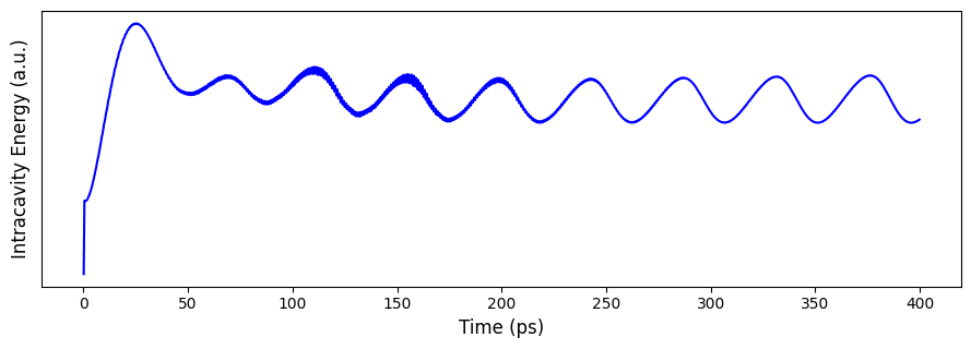
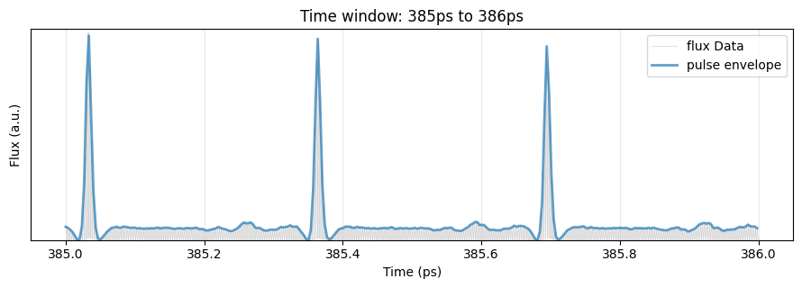
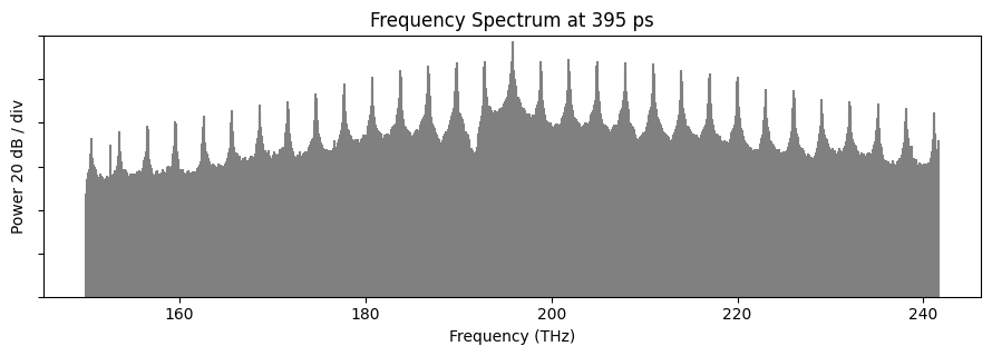
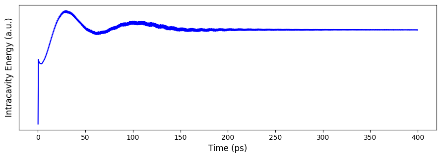
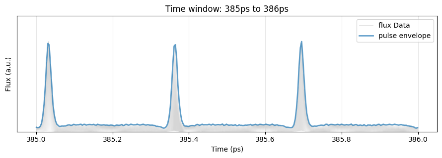
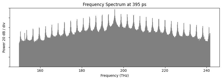
The intracavity energy quickly reaches a steady state, indicating that the frequency-comb signal has entered a stable soliton regime. Subsequently, we observe temporally stable soliton pulses in the time domain, and a frequency comb whose spectral envelope is well approximated by a $\mathrm{sech}^2$ profile.
simdata_soliton_flux = sim_data.monitor_data["ring_flux"].flux * -1
plot_roundtrip_flux(simdata_soliton_flux)


plot_time_window_maxima(simdata_soliton_flux, 385e-12, 386e-12, ylim=(0, 5e4))


# Call the function
monitor = sim_data.monitor_data["ring_mode"]
plot_frequency_spectrum(monitor, time_ps=395)
Breathing Soliton
By simply tuning the pump conditions, we can shift the operating point into the breathing-soliton regime.
breathing_freq0 = 195.83e12
breathing_amp = 28

breathing_mode_source = td.ModeSource(
    size=mode_plane.size,
    center=mode_plane.center,
    source_time=td.ContinuousWave(
        freq0=breathing_freq0, fwidth=fwidth, amplitude=breathing_amp
    ),
    mode_spec=td.ModeSpec(num_modes=2),
    mode_index=1,
    direction="+",
    num_freqs=11,
)

sim_breathing = sim.updated_copy(sources=[breathing_mode_source, pulse_source])

sim_breathing_data = web.run(
    sim_breathing,
    task_name="2DKerrBreathingSoliton",
    path="data/simulation_data_breathing.hdf5",
    verbose=True,
)
14:36:35 -03 WARNING: A large number (2001) of frequencies detected in monitor
             'ring_mode'. This can lead to solver slow-down and increased cost.
             Consider decreasing the number of frequencies in the monitor. This
             may become a hard limit in future Tidy3D versions.
             WARNING: Simulation has 5.06e+06 time steps. The 'run_time' may be
             unnecessarily large, unless there are very long-lived resonances.
             Created task '2DKerrBreathingSoliton' with task_id
             'fdve-18141984-a0ba-4b09-a3ec-1df65515a4ae' and task_type 'FDTD'.
             View task using web UI at
             'https://tidy3d.simulation.cloud/workbench?taskId=fdve-18141984-a0b
             a-4b09-a3ec-1df65515a4ae'.
Task folder: 'default'.
Output()
14:36:38 -03 Maximum FlexCredit cost: 3.377. Minimum cost depends on task
             execution details. Use 'web.real_cost(task_id)' to get the billed
             FlexCredit cost after a simulation run.
14:36:39 -03 status = queued
             To cancel the simulation, use 'web.abort(task_id)' or
             'web.delete(task_id)' or abort/delete the task in the web UI.
             Terminating the Python script will not stop the job running on the
             cloud.
Output()
14:36:51 -03 status = preprocess
14:37:57 -03 starting up solver
running solver
Output()
15:17:38 -03 status = postprocess
Output()
15:17:42 -03 status = success
15:17:44 -03 View simulation result at
             'https://tidy3d.simulation.cloud/workbench?taskId=fdve-18141984-a0b
             a-4b09-a3ec-1df65515a4ae'.
Output()
15:18:10 -03 loading simulation from data/simulation_data_breathing.hdf5
             WARNING: A large number (2001) of frequencies detected in monitor
             'ring_mode'. This can lead to solver slow-down and increased cost.
             Consider decreasing the number of frequencies in the monitor. This
             may become a hard limit in future Tidy3D versions.
             WARNING: Warning messages were found in the solver log. For more
             information, check 'SimulationData.log' or use
             'web.download_log(task_id)'.
In this case, the intracavity energy exhibits periodic modulation, and the soliton pulse amplitude in the time domain oscillates accordingly. The spectrum remains largely similar to that of a stationary soliton, with the envelope showing slight variations.
simdata_breathing_soliton_flux = sim_breathing_data.monitor_data["ring_flux"].flux * -1
plot_roundtrip_flux(simdata_breathing_soliton_flux)
plot_time_window_maxima(
    simdata_breathing_soliton_flux, 385e-12, 386e-12, ylim=(0, 0.92e5)
)


# Call the function
breathing_monitor = sim_breathing_data.monitor_data["ring_mode"]
plot_frequency_spectrum(breathing_monitor, time_ps=395)