Author: Dr. Zhiyi Yuan, Nayang Technological University.
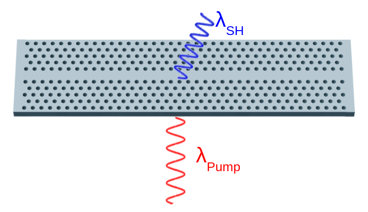
This notebook reproduces the paper: "Vertical chiral emission from an intrinsically achiral metasurface enabled with anisotropic continuum".
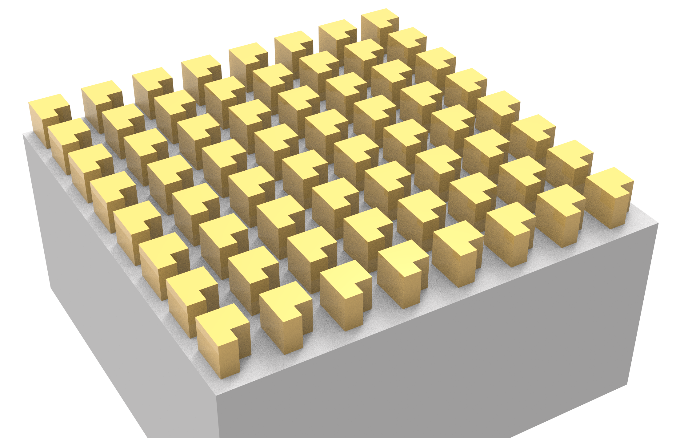
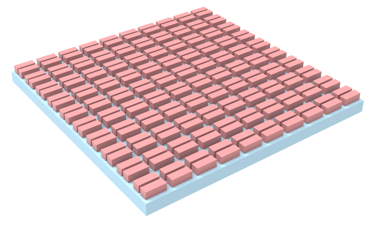
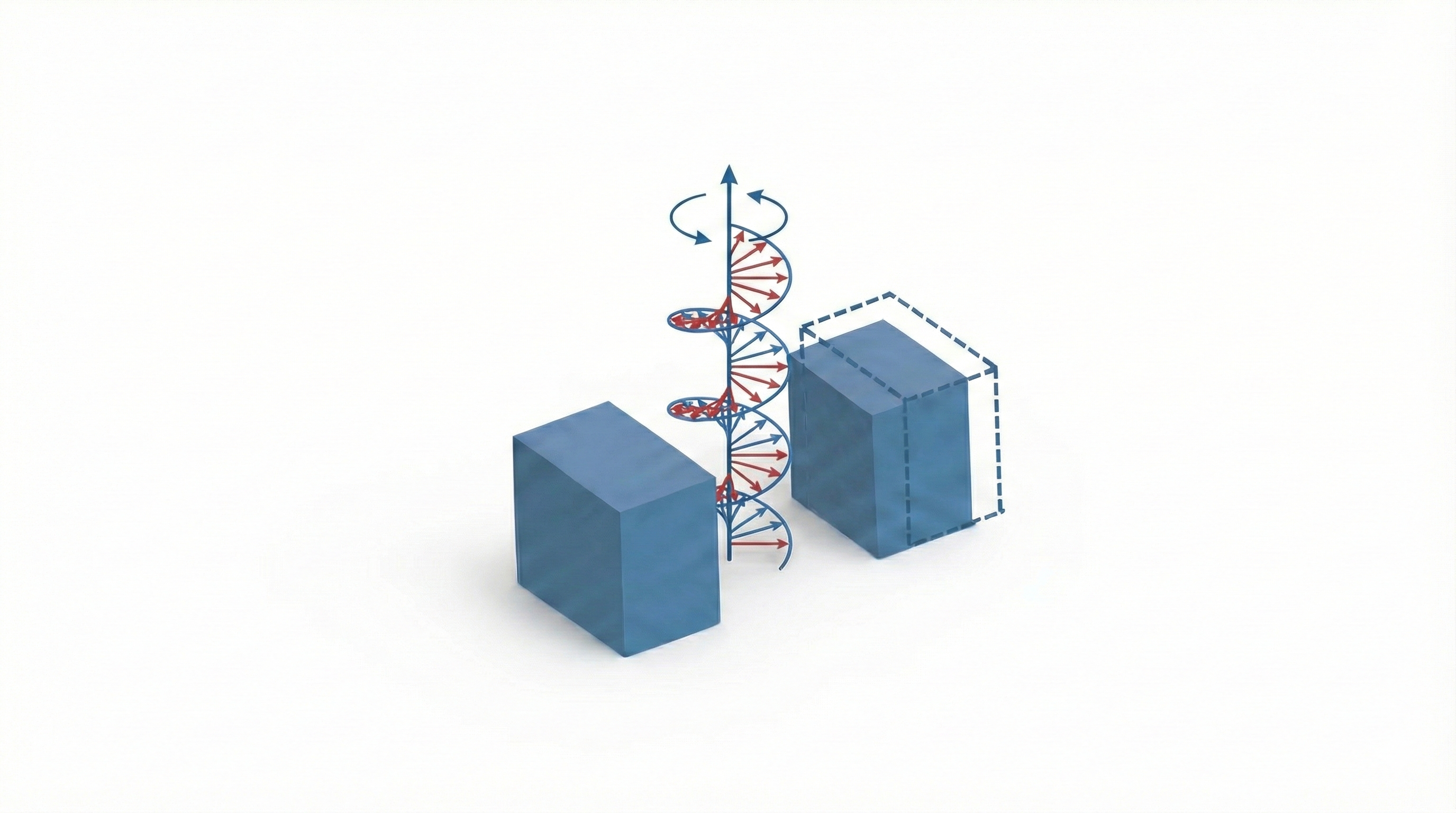
In particular, we simulate the unit cell of a $\sigma_z$-symmetric dielectric metasurface. We create a silicon dimer in PMMA with symmetry offset by parameters $\alpha$ and $\delta t$ in location and size. We reproduce the reflectance spectra for $\alpha$ = 0.09 and $\delta t$ = 11 nm, as well as the transmission spectra of the metasurface for TE and TM incidence in the xz plane.
import matplotlib.pyplot as plt
import numpy as np
import tidy3d as td
import tidy3d.web as web
from tidy3d.plugins.dispersion import FastDispersionFitter
from matplotlib.patches import Rectangle
import os
21:56:39 EST WARNING: Configuration found in legacy location '~/.tidy3d'.
             Consider running 'tidy3d config migrate'.
Create Structures in Unit Cell
P = 0.35
L = 0.19
W = 0.09
H = 0.21
delta = 0.011
alpha = 0.09
lba = 0.75
medium_structure = td.Medium(permittivity=3.90**2)
medium_env = td.Medium(permittivity=1.45**2)

box_1 = td.Box(center=(-P/4, 0, 0), size=(W, L, H))
box_2 = td.Box(center=(P/4-delta, -L*alpha/2, 0), size=(W, L*(1-alpha), H))
# create the chiral structure
metasurface_geom = td.GeometryGroup(geometries=[box_1, box_2])
metasurface_structure = td.Structure(geometry=metasurface_geom, medium=medium_structure)
# create the substrate structure
inf_eff = 1e2
#substrate = td.Structure(
#    geometry=td.Box(center=(0, 0, -H/2-lda/2), size=(td.inf, td.inf, lba)),
#    medium=medium_env,
#)
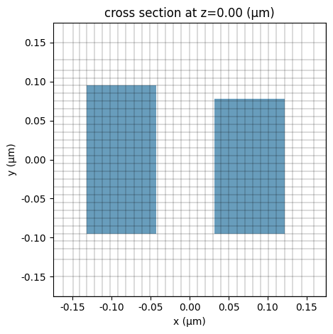
Create First Simulations
Here we create two simulations to measure the reflectance spectra for both x-polarized and y-polarized radiation.
lda_start = 0.7
lda_end = 0.9
n_freqs = 1001
ldas = np.linspace(lda_start, lda_end, n_freqs)
freqs = td.C_0 / ldas
freq0 = td.C_0 / np.mean(ldas)
fwidth = 0.5 * (np.max(freqs) - np.min(freqs))
run_time = 3e-12
monitor_z = 1  # monitor z position
flux_monitor = td.FluxMonitor(
    center=[0, 0, -monitor_z], size=[td.inf, td.inf, 0], freqs=freqs, name="flux"
)
source_z = 1
# create an oblique plane wave source
plane_wave_x = td.PlaneWave(
    center=[0, 0, source_z],
    size=[td.inf, td.inf, 0],
    source_time=td.GaussianPulse(freq0=freq0, fwidth=fwidth, phase=0.0),
    direction="-",
    angle_theta=0,
    angle_phi=0,
    pol_angle=0,
    #angular_spec=td.FixedInPlaneKSpec(),
)

plane_wave_y = td.PlaneWave(
    center=[0, 0, source_z],
    size=[td.inf, td.inf, 0],
    source_time=td.GaussianPulse(freq0=freq0, fwidth=fwidth, phase=0.0),
    direction="-",
    angle_theta=0,
    angle_phi=0,
    pol_angle=np.pi/2,
    #angular_spec=td.FixedInPlaneKSpec(),
)

# construct simulation
sim = td.Simulation(
    center=(0,0,0),
    size=(P, P, 3),
    grid_spec=td.GridSpec.auto(min_steps_per_wvl=20, max_scale=1.5),
    structures=[metasurface_structure],
    sources=[plane_wave_x],
    monitors=[flux_monitor],
    run_time=run_time,
    boundary_spec=td.BoundarySpec(
        x=td.Boundary.periodic(),
        y=td.Boundary.periodic(),
        z=td.Boundary.pml(),),
    medium=medium_env,
    shutoff=1e-5,
)

#ax = sim.plot(z=h/2)
#sim.plot_grid(z=h/2, ax=ax)
#plt.show()
#sim.plot_3d()
ax = sim.plot(z=0)
sim.plot_grid(z=0, ax=ax)
plt.show()
Run the simulations. The final field decay value will be small but above our automatic shutoff value of 1e-5, which will throw some warnings. This will have a negligible effect, so for demonstration purposes we will suppress the warnings.
td.config.logging.level = "ERROR"
sim_data_x = td.web.run(sim,task_name="VerticalChiral_X",verbose=True)

sim_data_y = sim.copy(update={"sources": [plane_wave_y]})
sim_data_y = td.web.run(sim_data_y,task_name="VerticalChiral_Y",verbose=True)
21:56:41 EST Created task 'VerticalChiral_X' with resource_id
             'fdve-93e9dab4-c821-4e22-a710-df130b4a7a41' and task_type 'FDTD'.
             View task using web UI at
             'https://tidy3d.simulation.cloud/workbench?taskId=fdve-93e9dab4-c82
             1-4e22-a710-df130b4a7a41'.
Task folder: 'default'.
Output()
21:56:43 EST Estimated FlexCredit cost: 0.025. Minimum cost depends on task
             execution details. Use 'web.real_cost(task_id)' to get the billed
             FlexCredit cost after a simulation run.
21:56:45 EST status = success
Output()
21:56:46 EST Loading simulation from simulation_data.hdf5
             Created task 'VerticalChiral_Y' with resource_id
             'fdve-3a075e0a-0542-4027-84b2-9da4639aeb5d' and task_type 'FDTD'.
             View task using web UI at
             'https://tidy3d.simulation.cloud/workbench?taskId=fdve-3a075e0a-054
             2-4027-84b2-9da4639aeb5d'.
Task folder: 'default'.
Output()
21:56:48 EST Estimated FlexCredit cost: 0.025. Minimum cost depends on task
             execution details. Use 'web.real_cost(task_id)' to get the billed
             FlexCredit cost after a simulation run.
21:56:49 EST status = success
Output()
21:56:50 EST Loading simulation from simulation_data.hdf5
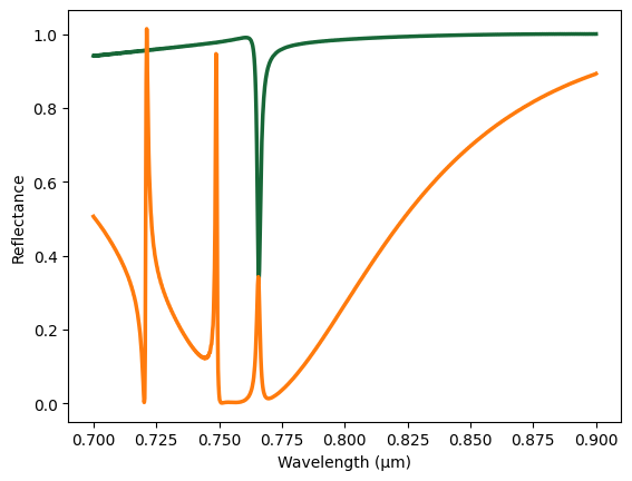
Visualize the reflectance.
monitor_data_lcp = sim_data_x.monitor_data
monitor_data_rcp = sim_data_y.monitor_data
T_lcp = monitor_data_lcp["flux"].flux
T_rcp = monitor_data_rcp["flux"].flux
plt.plot(ldas, -T_lcp, linewidth=2.5, label="LCP")
plt.plot(ldas, -T_rcp, linewidth=2.5, label="RCP")
plt.xlabel("Wavelength (μm)")
plt.ylabel("Reflectance")
plt.show()
Create Simulation Batch for TM Transmission
Where the input plane wave radiation is P-polarized.
def make_sim(theta):
    # create a plane wave source
    source_z = 0.6
    # create an oblique plane wave source
    plane_wave_x = td.PlaneWave(
        center=[0, 0, source_z],
        size=[td.inf, td.inf, 0],
        source_time=td.GaussianPulse(freq0=freq0, fwidth=fwidth),
        direction="-",
        angle_theta=theta,
        angle_phi=0,
        pol_angle=0,
        angular_spec=td.FixedInPlaneKSpec()
    )

    # construct simulation
    sim = td.Simulation(
        size=(P, P, 3),
        grid_spec=td.GridSpec.auto(min_steps_per_wvl=20, max_scale=1.5),
        structures=[metasurface_structure],
        sources=[plane_wave_x],
        monitors=[flux_monitor],
        run_time=run_time,
        boundary_spec=td.BoundarySpec(
            x=td.Boundary.bloch_from_source(source=plane_wave_x, domain_size=P, axis=0, medium=medium_env),
            y=td.Boundary.bloch_from_source(source=plane_wave_x, domain_size=P, axis=1, medium=medium_env),
            z=td.Boundary.pml(),
        ),
        medium=medium_env,
        shutoff=1e-5,
    )

    return sim
theta_list = np.linspace(-18, 18, 36)  # theta values for the parameter sweep
# create a dictionary of simulations
sims = {f"theta={theta:.1f}": make_sim(np.deg2rad(theta)) for theta in theta_list}
# create and run a batch of simulations
batch = web.Batch(simulations=sims)
batch_results = batch.run()
Output()
21:56:59 EST Started working on Batch containing 36 tasks.
21:57:32 EST Maximum FlexCredit cost: 0.900 for the whole batch.
             Use 'Batch.real_cost()' to get the billed FlexCredit cost after
             completion.
Output()
21:58:19 EST Batch complete.
T = np.array(
    [np.abs(batch_results[f"theta={theta:.1f}"]["flux"].flux.values) for theta in theta_list]
)
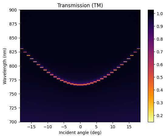
Transmission spectra of the metasurface for TM incidence. Under TM-polarized incidence, we can see that only the TM$_1$ mode is excited, as opposed to the TE incidence simulated below.
plt.pcolormesh(theta_list,ldas*1e3,T.T, cmap="inferno_r")
plt.ylabel("Wavelength (nm)")
plt.xlabel("Incident angle (deg)")
plt.title("Transmission (TM)")
plt.colorbar()
plt.show()
Create Simulation Batch for TE Transmission
Where the input plane wave radiation is S-polarized.
def make_sim(theta):
    # create a plane wave source
    source_z = 0.6
    # create an oblique plane wave source
    plane_wave_y = td.PlaneWave(
        center=[0, 0, source_z],
        size=[td.inf, td.inf, 0],
        source_time=td.GaussianPulse(freq0=freq0, fwidth=fwidth),
        direction="-",
        angle_theta=theta,
        angle_phi=0,
        pol_angle=np.pi/2,
        angular_spec=td.FixedInPlaneKSpec(),
    )

    # construct simulation
    sim = td.Simulation(
        size=(P, P, 3),
        grid_spec=td.GridSpec.auto(min_steps_per_wvl=20, max_scale=1.5),
        structures=[metasurface_structure],
        sources=[plane_wave_y],
        monitors=[flux_monitor],
        run_time=run_time,
        boundary_spec=td.BoundarySpec(
            x=td.Boundary.bloch_from_source(source=plane_wave_y, domain_size=P, axis=0, medium=medium_env),
            y=td.Boundary.bloch_from_source(source=plane_wave_y, domain_size=P, axis=1, medium=medium_env),
            z=td.Boundary.pml(),
        ),
        medium=medium_env,
        shutoff=1e-5,
    )

    return sim
theta_list = np.linspace(-18, 18, 36)  # theta values for the parameter sweep
# create a dictionary of simulations
sims = {f"theta={theta:.1f}": make_sim(np.deg2rad(theta)) for theta in theta_list}
# create and run a batch of simulations
batch = web.Batch(simulations=sims)
batch_results = batch.run()
Output()
21:58:51 EST Started working on Batch containing 36 tasks.
21:59:24 EST Maximum FlexCredit cost: 0.900 for the whole batch.
             Use 'Batch.real_cost()' to get the billed FlexCredit cost after
             completion.
Output()
22:00:11 EST Batch complete.
T = np.array(
    [np.abs(batch_results[f"theta={theta:.1f}"]["flux"].flux.values) for theta in theta_list]
)
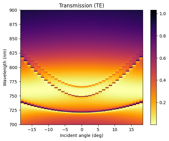
Transmission spectra of the metasurface for TE incidence. Under TE-polarized incidence, we can see 3 modes: TM$_1$, TE$_1$, and TM$_2$. The TM$_1$ mode has a dip in transmission, expected by the paper through coupling to the TM and TE components.
plt.pcolormesh(theta_list,ldas*1e3,T.T, cmap="inferno_r")
plt.ylabel("Wavelength (nm)")
plt.xlabel("Incident angle (deg)")
plt.title("Transmission (TE)")
plt.colorbar()
plt.show()