TIDY3D
LEARNING CENTER

Lectures

Tutorials

Applications

Parameter sweep in RF simulation¶

This notebook demonstrates how to perform parameter sweeps in RF simulations. Individual RF simulations are defined by TerminalComponentModeler (TCM) objects. To define a batch job, we simply construct a dictionary of TCM objects where each (key, value) pair contains a user-defined text label and the corresponding TCM object. Then, we use the usual web.run() command to submit this dict object instead of a single TCM.

There are many different methods to generate the dictionary of TCM simulations. For basic parameter sweeps, one can define a parametric wrapper function to build the TCM for a given parameter value set. Then, use a basic for loop to iteratively build the dictionary. This workflow is demonstrated below. After the batch simulations are completed, we also demonstrate how to access the S-parameter and field monitor data.

The workflow extends very easily to other design space exploration (DSE) algorithms. Simply replace the basic for loop with the appropriate logic for the DSE algorithm.

[1]:

import matplotlib.pyplot as plt
import numpy as np
import tidy3d as td
import tidy3d.rf as rf
import tidy3d.web as web

td.config.logging.level = "ERROR"

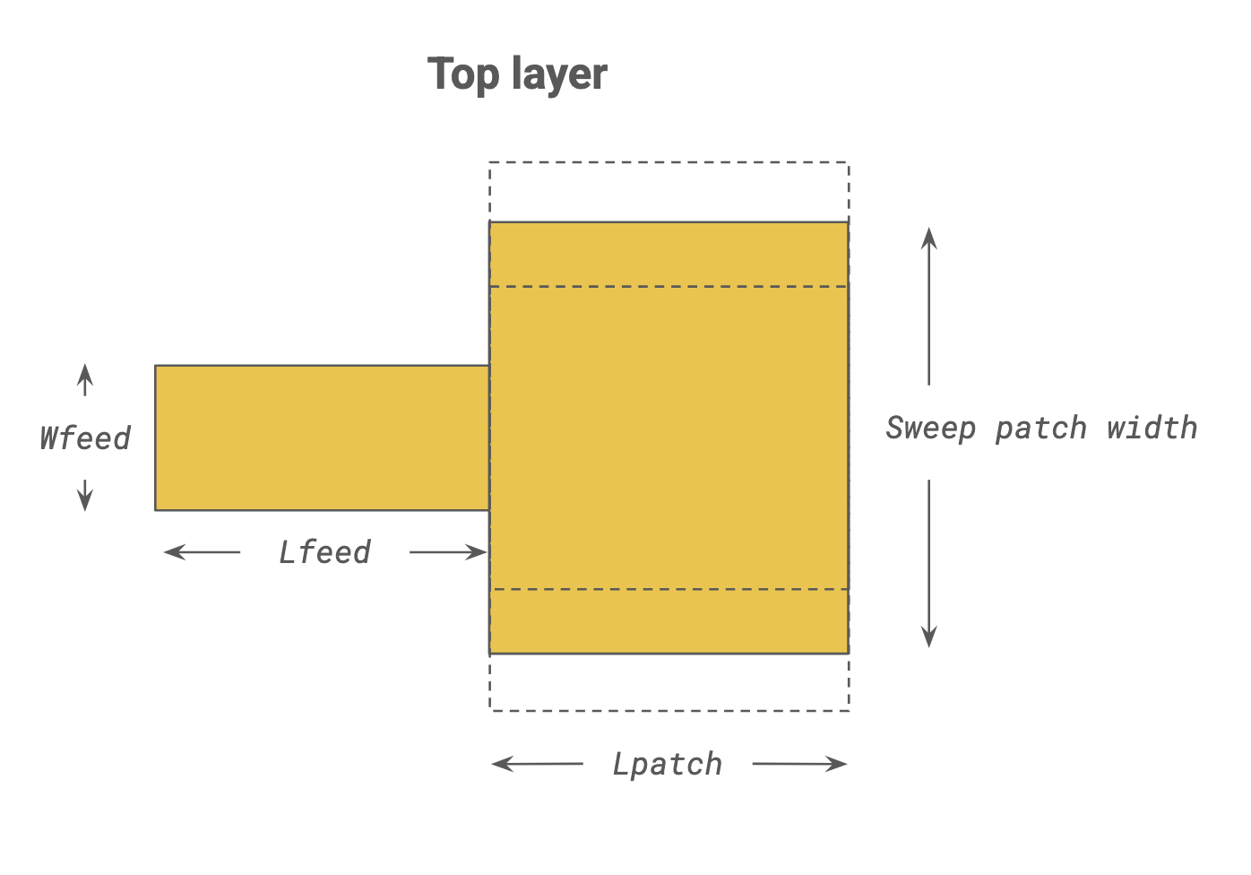
Below, we set up some of the basic parameters of this demo. We will be constructing an edge-fed metal patch, and sweeping the width (y length) of the patch.

No description has been provided for this image

[2]:

# Frequency range
f_min, f_max = (1e9, 20e9)
f0 = (f_max + f_min) / 2
freqs = np.linspace(f_min, f_max, 601)

# Geometry dimensions
mm = 1000
Lsub, Wsub = (20 * mm, 20 * mm)  # substrate dimensions
Hsub = 1.5 * mm  # substrate thickness
Hmetal = 0.035 * mm  # metal thickness
Lpatch = 8 * mm  # patch dimensions
Lfeed, Wfeed = ((Lsub - Lpatch) / 2, 2.9 * mm)  # feedline size

# Materials
metal = rf.LossyMetalMedium(conductivity=58, frequency_range=(f_min, f_max))
dielectric = td.Medium(permittivity=4.3)

Defining a Parametric Wrapper Function¶

Instead of defining a static TerminalComponentModeler, we define a wrapper function build_tcm() that dynamically generates the TCM for a given patch_width.

[3]:

# Parametric function that generates a TerminalComponentModeler (TCM)
def build_tcm(patch_width):
    # Build structures
    substrate = td.Structure(
        geometry=td.Box(center=(0, 0, -Hsub / 2), size=(Lsub, Wsub, Hsub)), medium=dielectric
    )
    ground = td.Structure(
        geometry=td.Box(center=(0, 0, -Hsub - Hmetal / 2), size=(Lsub, Wsub, Hmetal)), medium=metal
    )
    feed = td.Structure(
        geometry=td.Box(
            center=(-Lpatch / 2 - Lfeed / 2, 0, Hmetal / 2), size=(Lfeed, Wfeed, Hmetal)
        ),
        medium=metal,
    )

    # Build patch (note use of input parameter patch_width)
    patch = td.Structure(
        geometry=td.Box(center=(0, 0, Hmetal / 2), size=(Lpatch, patch_width, Hmetal)), medium=metal
    )

    # Define port
    LP1 = rf.LumpedPort(
        center=(-Lsub / 2, 0, -Hsub / 2), size=(0, Wfeed, Hsub), voltage_axis=2, name="LP1"
    )

    # Define field monitor
    mon_1 = td.FieldMonitor(size=(td.inf, td.inf, 0), freqs=[f0], name="field (z=0)")

    # Define layer refinement
    lr_options = {
        "min_steps_along_axis": 1,
        "corner_refinement": td.GridRefinement(dl=0.15 * mm, num_cells=2),
    }
    layer_ref_1 = rf.LayerRefinementSpec.from_structures(structures=[feed, patch], **lr_options)
    layer_ref_2 = rf.LayerRefinementSpec.from_structures(structures=[ground], **lr_options)

    # Define grid
    grid_spec = td.GridSpec.auto(
        wavelength=td.C_0 / f0,
        min_steps_per_wvl=20,
        layer_refinement_specs=[layer_ref_1, layer_ref_2],
    )

    # Define simulation and TCM
    sim = td.Simulation(
        size=(30 * mm, 30 * mm, 8 * mm),
        structures=[substrate, ground, feed, patch],
        monitors=[mon_1],
        grid_spec=grid_spec,
        run_time=5e-9,
        plot_length_units="mm",
    )
    tcm = rf.TerminalComponentModeler(simulation=sim, ports=[LP1], freqs=freqs)

    # Return TCM object
    return tcm

Generate Batch Dictionary¶

Using build_tcm(), we iteratively construct a dictionary dict_tcm, whose (key, value) pairs are given by a user-defined text label from sweep_labels and the respective TCM instance.

[4]:

# Generate list of sweep values and corresponding labels
sweep_values = np.linspace(10 * mm, 12 * mm, 3)
sweep_labels = [f"patch_width={val / mm:.1f}mm" for val in sweep_values]

# Iteratively generate dict for batch job
dict_tcm = {}
for label, val in zip(sweep_labels, sweep_values):
    dict_tcm[label] = build_tcm(patch_width=val)

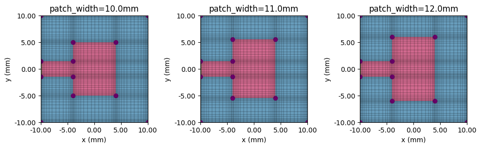
Before running, we can iterate over dict_tcm to inspect individual jobs.

[5]:

fig, ax = plt.subplots(1, 3, figsize=(10, 6), tight_layout=True)
for ii, (label, tcm_plot) in enumerate(dict_tcm.items()):
    tcm_plot.plot_sim(z=0, ax=ax[ii], monitor_alpha=0)
    tcm_plot.simulation.plot_grid(z=0, ax=ax[ii])
    ax[ii].set_xlim(-Lsub / 2, Lsub / 2)
    ax[ii].set_ylim(-Wsub / 2, Wsub / 2)
    ax[ii].set_title(label)
plt.show()

Submit Batch Job¶

We use the web.run() method to initiate the job. The syntax for submitting a batch TCM job is identical to that of submitting a single TCM job.

[6]:

# Submit batch job
batch_tcm_data = web.run(dict_tcm, task_name="RF parameter sweep demo", path="./data")

Output()

15:49:08 EST Started working on Batch containing 3 tasks.

15:49:17 EST Maximum FlexCredit cost: 0.075 for the whole batch.

             Use 'Batch.real_cost()' to get the billed FlexCredit cost after    
             completion.

Output()

15:50:13 EST Batch complete.

Process Batch Results¶

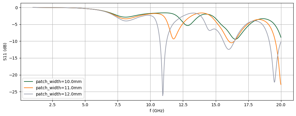
After a successful batch run, we use the returned dict object batch_tcm_data to access the result data. Its structure mirrors that of the dictionary dict_tcm that generated it - that is, one can access the individual job data using the same key label tcm_data = batch_tcm_data[key_label]. One can also iterate over all batch data using the batch_tcm_data.items() iterator, demonstrated below.

[7]:

# Plot S11 comparison
fig, ax = plt.subplots(figsize=(10, 4), tight_layout=True)
for label, tcm_data_iter in batch_tcm_data.items():
    # Get S11 in dB
    S11 = tcm_data_iter.smatrix().data.squeeze()
    S11dB = 20 * np.log10(np.abs(S11))
    # Plot S11
    ax.plot(freqs / 1e9, S11dB, label=label)
ax.legend()
ax.grid()
ax.set_xlabel("f (GHz)")
ax.set_ylabel("S11 (dB)")
plt.show()

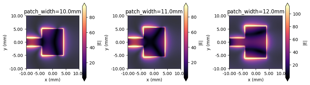
One can follow a similar process to access FieldMonitor data if present in the simulation.

[8]:

# Plot field monitor results
fig, ax = plt.subplots(1, 3, figsize=(10, 3), tight_layout=True)
for ii, (label, tcm_data_iter) in enumerate(batch_tcm_data.items()):
    sim_data = tcm_data_iter.data["LP1"]  # Get simulation data from port 1 excitation
    sim_data.plot_field("field (z=0)", field_name="E", val="abs", ax=ax[ii])
    ax[ii].set_xlim(-Lsub / 2, Lsub / 2)
    ax[ii].set_ylim(-Lsub / 2, Lsub / 2)
    ax[ii].set_title(label)
plt.show()

[ ]:

Example library

Previous Tutorial Next Tutorial

TIDY3D LEARNING CENTER