The power divider is a key component in modern wireless communications systems. It is usually subject to key performance metrics such as low insertion loss, minimal crosstalk between output ports, and a small footprint. In addition, low pass or bandpass filters are typically incorporated in order to suppress unwanted harmonics and noise in wireless signals. These filters should have a sharp response, quantified by the roll-off rate (ROR), and a wide stopband.
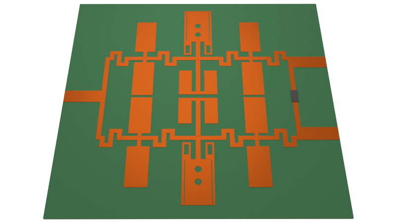
In this 3-part notebook series, we will simulate various stages of the design process of a Wilkinson power divider (WPD) created by Moloudian et al in [1].
- In part one (this notebook), we start with a simple low pass filter design and improve its filter response in order to achieve a higher roll-off rate (ROR).
- In part two, we will add a harmonic suppression circuit to the low pass filter to achieve a wide stopband.
- In part three, we will implement the full WPD design and compare its performance to a conventional WPD.
import matplotlib.pyplot as plt
import numpy as np
import tidy3d as td
import tidy3d.rf as rf
from tidy3d.plugins.dispersion import FastDispersionFitter

td.config.logging.level = "ERROR"
General Parameters and Mediums
The target cutoff frequency of the low pass filter is 1.8 GHz (within the GSM band) and the simulation will cover 0.1 to 8 GHz. The bandwidth of the simulation is defined using the FreqRange utility class.
(f_min, f_max) = (0.1e9, 8e9)
bandwidth = td.FreqRange.from_freq_interval(f_min, f_max)
f0 = bandwidth.freq0
freqs = bandwidth.freqs(num_points=401)
The substrate is FR4 and the metallic traces are copper. We assume both materials have constant non-zero loss across the bandwidth: loss tangent of 0.022 for FR4 and conductivity of 6E7 S/m (i.e. 60 S/um) for copper.
med_FR4 = FastDispersionFitter.constant_loss_tangent_model(4.4, 0.022, (f_min, f_max))
med_Cu = rf.LossyMetalMedium(conductivity=60, frequency_range=(f_min, f_max))
Basic resonator
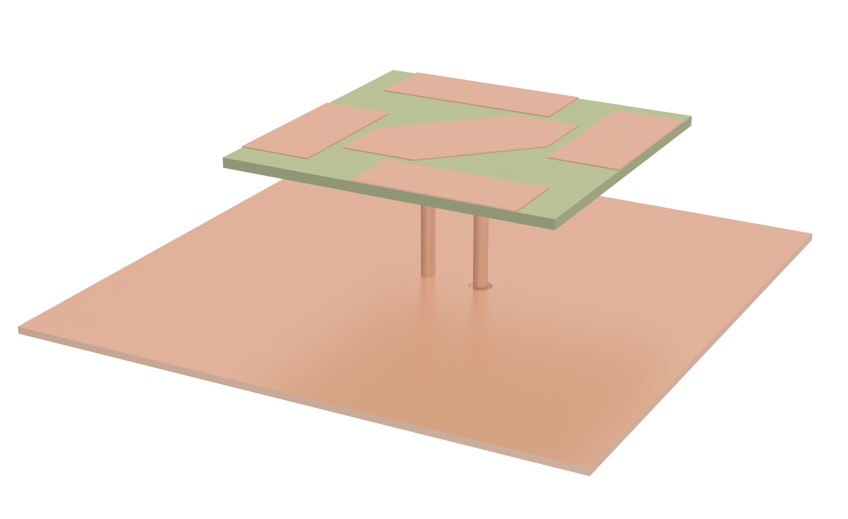
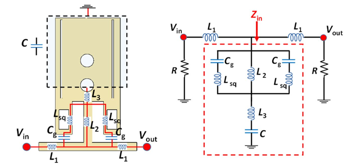
The basic low pass filter uses a LC resonator design shown below. The geometric lengths and widths of each metallic patch determines its equivalent inductance and capacitance.
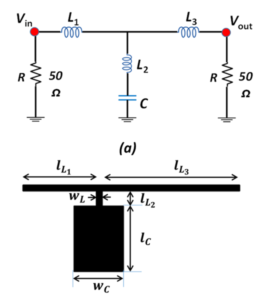
The figure above is taken from Figure 2 in [1].
Geometry and Structure
Using the dimensions provided in [1], we recreate the resonator structure below.
# Geometry dimensions
mm = 1000  # Conversion factor micron to mm
H = 0.8 * mm  # Substrate thickness
T = 0.035 * mm  # Metal thickness
WL = 0.5 * mm  # Line width
LL1, LL2, LL3 = (5.8 * mm, 1.2 * mm, 11.1 * mm)  # Line lengths
WC, LC = (4 * mm, 5.3 * mm)  # Patch dimensions
Lsub, Wsub = (LL1 + WL + LL3, 2 * (LC + WL + LL2))  # Substrate dimensions
# Resonator geometry
geom_C = td.Box.from_bounds(rmin=(-WC / 2, 0, 0), rmax=(WC / 2, LC, T))
geom_L2 = td.Box.from_bounds(rmin=(-WL / 2, -LL2 - WL, 0), rmax=(WL / 2, 0, T))
geom_L1 = td.Box.from_bounds(rmin=(-WL / 2 - LL1, -LL2 - WL, 0), rmax=(-WL / 2, -LL2, T))
geom_L3 = td.Box.from_bounds(rmin=(WL / 2, -LL2 - WL, 0), rmax=(WL / 2 + LL3, -LL2, T))
geom_resonator_basic = td.GeometryGroup(geometries=[geom_C, geom_L1, geom_L2, geom_L3])

# Substrate and ground plane geometry
x0, y0, z0 = geom_resonator_basic.bounding_box.center  # center (x,y) with circuit
geom_gnd = td.Box(center=(x0, y0, -H - T / 2), size=(Lsub, Wsub, T))
geom_sub = td.Box(center=(x0, y0, -H / 2), size=(Lsub, Wsub, H))
# create structures
str_sub = td.Structure(geometry=geom_sub, medium=med_FR4)
str_gnd = td.Structure(geometry=geom_gnd, medium=med_Cu)
str_resonator_basic = td.Structure(geometry=geom_resonator_basic, medium=med_Cu)

str_list_basic = [str_sub, str_gnd, str_resonator_basic]  # List of structures
Monitors and Ports
We define an in-plane field monitor for visualization purposes.
# Field Monitors
mon_1 = td.FieldMonitor(
    center=(0, 0, 0),
    size=(td.inf, td.inf, 0),
    freqs=[f_min, f0, f_max],
    name="field in-plane",
)
The structure is terminated with two 50 ohm lumped ports.
# Lumped port
lp_options = {"size": (0, WL, H), "voltage_axis": 2, "impedance": 50}
LP1 = rf.LumpedPort(center=(-WL / 2 - LL1, -WL / 2 - LL2, -H / 2), name="LP1", **lp_options)
LP2 = rf.LumpedPort(center=(WL / 2 + LL3, -WL / 2 - LL2, -H / 2), name="LP2", **lp_options)
port_list = [LP1, LP2]  # List of ports
Grid and Boundary
By default, the simulation boundary is open (PML) on all sides. We add quarter-wavelength padding on all sides to ensure the boundaries do not encroach on the near-field.
# Add padding
padding = td.C_0 / f0 / 2
sim_LX = Lsub + padding
sim_LY = Wsub + padding
sim_LZ = H + padding
We use LayerRefinementSpec to automatically refine the grid along corners and edges of the metallic resonator. The rest of the grid is automatically created with the minimum grid size determined by the wavelength.
# Layer refinement on resonator
lr_spec = rf.LayerRefinementSpec.from_structures(
    structures=[str_resonator_basic],
    min_steps_along_axis=1,
    corner_refinement=td.GridRefinement(dl=T, num_cells=2),
)

# Define overall grid spec
grid_spec = td.GridSpec.auto(
    wavelength=td.C_0 / f0,
    min_steps_per_wvl=12,
    layer_refinement_specs=[lr_spec],
)
Simulation and TerminalComponentModeler
We define the Simulation and TerminalComponentModeler objects below. The latter facilitates a batch port sweep in order to compute the full S-parameter matrix.
# Define simulation object
sim = td.Simulation(
    center=(x0, y0, z0),
    size=(sim_LX, sim_LY, sim_LZ),
    structures=str_list_basic,
    grid_spec=grid_spec,
    monitors=[mon_1],
    run_time=5e-9,
    plot_length_units="mm",
)
# Define TerminalComponentModeler
tcm = rf.TerminalComponentModeler(
    simulation=sim,
    ports=port_list,
    freqs=freqs,
    remove_dc_component=False,
)
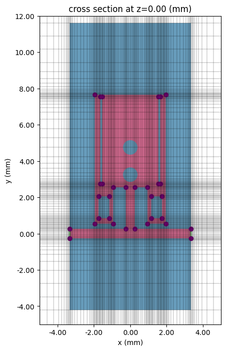
Visualization
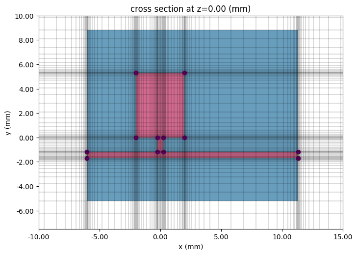
Before running, it is a good idea to check the structure layout and simulation grid.
# In-plane
fig, ax = plt.subplots(figsize=(8, 6))
tcm.plot_sim(z=0, ax=ax, monitor_alpha=0)
tcm.simulation.plot_grid(z=0, ax=ax, hlim=(-10 * mm, 15 * mm), vlim=(-7.5 * mm, 10 * mm))
plt.show()
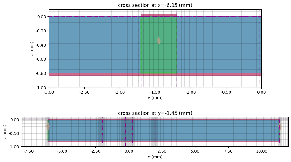
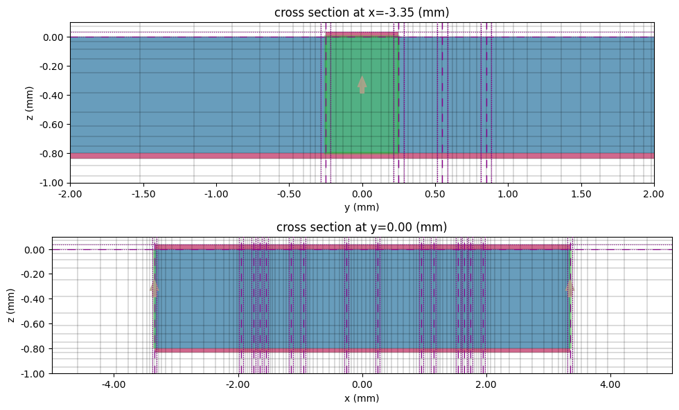
# Cross section and port
fig, ax = plt.subplots(2, 1, figsize=(10, 6), tight_layout=True)
tcm.plot_sim(x=-LL1 - WL / 2, ax=ax[0], monitor_alpha=0)
tcm.simulation.plot_grid(
    x=-LL1 - WL / 2, ax=ax[0], hlim=(-3 * mm, 0 * mm), vlim=(-1 * mm, 0.1 * mm)
)
tcm.plot_sim(y=-LL2 - WL / 2, ax=ax[1], monitor_alpha=0)
tcm.simulation.plot_grid(
    y=-LL2 - WL / 2, ax=ax[1], hlim=(-8 * mm, 12 * mm), vlim=(-1 * mm, 0.1 * mm)
)
ax[1].set_aspect(2)
plt.show()
Running the Simulation
The tidy3d.web.run() method executes the job and downloads the simulation data after completion.
tcm_data_basic = td.web.run(tcm, task_name="WPD basic resonator", path="data/tcm_data_basic.hdf5")
16:40:47 EST Created task 'WPD basic resonator' with resource_id
             'sid-b1ee4ada-11f5-4d18-b026-3ff9fd697543' and task_type
             'TERMINAL_CM'.
             View task using web UI at
             'https://tidy3d.simulation.cloud/rf?taskId=pa-2c140dfc-f64b-420b-b7
             f0-102a829ab8f9'.
Task folder: 'default'.
16:40:56 EST Maximum FlexCredit cost: 0.142. Minimum cost depends on task
             execution details. Use 'web.real_cost(task_id)' after run.
16:40:57 EST Subtasks status - WPD basic resonator
             Group ID: 'pa-2c140dfc-f64b-420b-b7f0-102a829ab8f9'
Batch status = preprocess
16:41:04 EST Batch status = running
16:41:44 EST Batch status = postprocess
16:41:55 EST Modeler has finished running successfully.
Billed flex credit cost: 0.050.
16:41:58 EST Loading component modeler data from data/tcm_data_basic.hdf5
Results
Field Profile
The TerminalComponentModelerData instance returned by tidy3d.web.run() stores the monitor data for each port in a dictionary in the data attribute. Use the corresponding port name to access it.
sim_data = tcm_data_basic.data["LP1"]
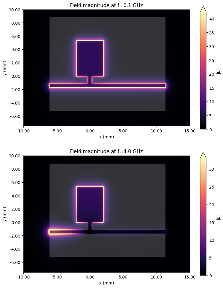
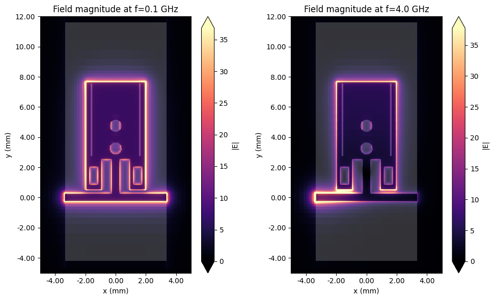
The in-plane field magnitude is plotted below at f_min and f0, showing a clear difference between the pass- and stopbands.
# Field plots
fig, ax = plt.subplots(2, 1, figsize=(8, 10), tight_layout=True)
sim_data.plot_field("field in-plane", "E", val="abs", f=f_min, ax=ax[0])
ax[0].set_title(f"Field magnitude at f={f_min / 1e9:.1f} GHz")
sim_data.plot_field("field in-plane", "E", val="abs", f=f0, ax=ax[1])
ax[1].set_title(f"Field magnitude at f={f0 / 1e9:.1f} GHz")
for axis in ax:
    axis.set_xlim(-10 * mm, 15 * mm)
    axis.set_ylim(-7.5 * mm, 10 * mm)
plt.show()
S-parameters
Use the smatrix() method to calculate the S-matrix.
smat = tcm_data_basic.smatrix()
We use the port_in and port_out coordinates to access the specific S-parameter from the full matrix. Note the use of np.conjugate() to convert from the default physics phase convention to the engineering convention.
S11 = np.conjugate(smat.data.isel(port_in=0, port_out=0))
S21 = np.conjugate(smat.data.isel(port_in=0, port_out=1))
S11dB = 20 * np.log10(np.abs(S11))
S21dB = 20 * np.log10(np.abs(S21))
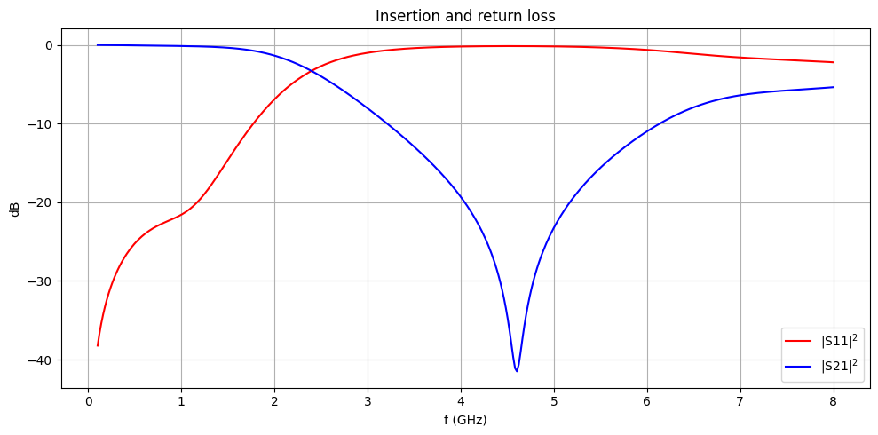
The insertion and return losses are plotted below.
fig, ax = plt.subplots(figsize=(10, 5), tight_layout=True)
ax.plot(freqs / 1e9, S11dB, "r", label="|S11|$^2$")
ax.plot(freqs / 1e9, S21dB, "b", label="|S21|$^2$")
ax.set_title("Insertion and return loss")
ax.set_xlabel("f (GHz)")
ax.set_ylabel("dB")
ax.legend()
ax.grid()
plt.show()
Roll-off rate
The roll-off rate (ROR) is a figure of merit that quantifies the sharpness of the filter response. It is calculated by $$ ROR = \frac{\Delta \alpha}{\Delta f} $$ where $\Delta \alpha$ is the difference in insertion loss (in dB) between two reference levels and $\Delta f$ is the corresponding difference in frequency. We choose -3 and -30 dB to be the two reference levels for this calculation.
def calculate_ROR(SdB):
    """Calculates ROR from input S-parameter (in dB)"""
    refdB_1 = -3
    refdB_2 = -30
    f1 = np.min(freqs[np.argsort(np.abs(SdB - refdB_1))][:2])
    f2 = np.min(freqs[np.argsort(np.abs(SdB - refdB_2))][:2])
    return (refdB_2 - refdB_1) / (f1 - f2) * 1e9  # in dB/GHz
print(f"ROR of basic LC resonator: {calculate_ROR(S21dB):.2f} dB/GHz")
ROR of basic LC resonator: 13.02 dB/GHz
Modified resonator
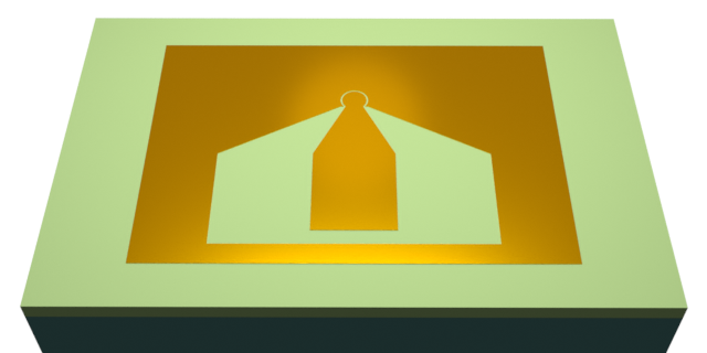
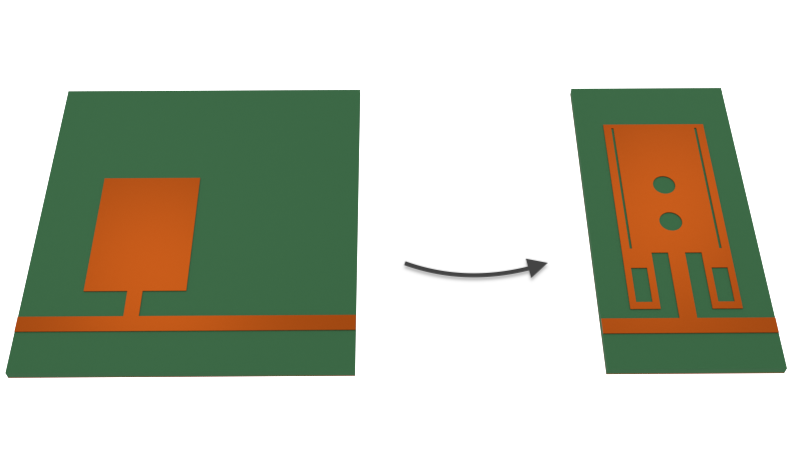
In the modified resonator, additional holes are cut into the resonator patch in order to create equivalent inductive and capacitive elements shown below. The patch is also adjusted to have a symmetric structure.
The figure above is taken from Figure 3 in [1].
Geometry and Structure
The dimensions of the resonator are mostly obtained from [1]. Missing dimensions are obtained via visual estimation.
# Modified resonator dimensions
MA, MB, MC, MD = (3.9 * mm, 7.1 * mm, 3.1 * mm, 2.3 * mm)
ME, MF, MG, MH = (0.6 * mm, 0.2 * mm, 1.2 * mm, 0.5 * mm)
MJ, MK, MM, MN = (4.8 * mm, 0.3 * mm, 0.1 * mm, 0.7 * mm)
MP, MQ, MR, MS = (0.1 * mm, 0.7 * mm, 0.4 * mm, 0.3 * mm)
Lsub2, Wsub2 = (2 * MC + MH, 2 * (MH + MK + MB))
The geometry and structures are created below. To "cut" holes in the patch resonator, we first create the hole geometry, then use the - operator apply the Boolean difference operation onto the main patch.
# Resonator geometry
geom_patch = td.Box.from_bounds(rmin=(-MA / 2, MH / 2 + MK, 0), rmax=(MA / 2, MH / 2 + MK + MB, T))
geom_hole1 = td.Box.from_bounds(
    rmin=(-MH / 2 - MN - MF - ME, MH / 2 + MK + MS, 0),
    rmax=(-MH / 2 - MN - MF, MH / 2 + MK + MS + MG, T),
)
geom_hole2 = geom_hole1.translated(2 * (MF + MN) + MH + ME, 0, 0)
geom_hole3 = td.Cylinder(center=(0, MH / 2 + MD + MQ, T / 2), radius=MR, length=T, axis=2)
geom_hole4 = geom_hole3.translated(0, MQ + 2 * MR, 0)
geom_hole5 = td.Box.from_bounds(
    rmin=(-MA / 2 + 1.5 * MF, MH / 2 + MK + MS + MG + MQ, 0),
    rmax=(-MA / 2 + 1.5 * MF + MM, MH / 2 + MK + MB - MP, T),
)
geom_hole6 = geom_hole5.translated(-2 * geom_hole5.center[0], 0, 0)
geom_hole7 = td.Box.from_bounds(
    rmin=(-MH / 2 - MN, MH / 2 + MK, 0), rmax=(MH / 2 + MN, MH / 2 + MD, T)
)
for hole in [geom_hole1, geom_hole2, geom_hole3, geom_hole4, geom_hole5, geom_hole6, geom_hole7]:
    geom_patch -= hole

geom_line1 = td.Box.from_bounds(rmin=(-MH / 2, MH / 2, 0), rmax=(MH / 2, MH / 2 + MD, T))
geom_line2 = td.Box.from_bounds(rmin=(-MH / 2 - MC, -MH / 2, 0), rmax=(MH / 2 + MC, MH / 2, T))
geom_resonator_modified = td.GeometryGroup(geometries=[geom_line1, geom_line2, geom_patch])

# Substrate and ground
x1, y1, z1 = geom_resonator_modified.bounding_box.center
geom_sub2 = td.Box(center=(x1, y1, -H / 2), size=(Lsub2, Wsub2, H))
geom_gnd2 = td.Box(center=(x1, y1, -H - T / 2), size=(Lsub2, Wsub2, T))

# Structures
str_resonator_modified = td.Structure(geometry=geom_resonator_modified, medium=med_Cu)
str_sub2 = td.Structure(geometry=geom_sub2, medium=med_FR4)
str_gnd2 = td.Structure(geometry=geom_gnd2, medium=med_Cu)
str_list_modified = [str_sub2, str_gnd2, str_resonator_modified]
Ports
As before, we use 50 ohm lumped ports to terminate both ends of the feed line. Their positions are slightly shifted to account for the modified geometry.
# Lumped port
lp_options = {"size": (0, MH, H), "voltage_axis": 2, "impedance": 50}
LP1 = rf.LumpedPort(center=(-MH / 2 - MC, 0, -H / 2), name="LP1", **lp_options)
LP2 = rf.LumpedPort(center=(MH / 2 + MC, 0, -H / 2), name="LP2", **lp_options)
port_list = [LP1, LP2]  # List of ports
Grid and Boundary
The grid and boundary specifications are largely unchanged from the previous section.
# Add padding
padding = td.C_0 / f0 / 2
sim_LX = Lsub2 + padding
sim_LY = Wsub2 + padding
sim_LZ = H + padding
# Layer refinement on resonator
lr_spec = rf.LayerRefinementSpec.from_structures(
    structures=[str_resonator_modified],
    min_steps_along_axis=1,
    corner_refinement=td.GridRefinement(dl=T, num_cells=2),
)

# Define overall grid spec
grid_spec = td.GridSpec.auto(
    wavelength=td.C_0 / f0,
    min_steps_per_wvl=12,
    layer_refinement_specs=[lr_spec],
)
Simulation and TerminalComponentModeler
The Simulation and TerminalComponentModeler objects are defined similarly to the previous section.
# Define simulation object
sim = td.Simulation(
    center=(x1, y1, z1),
    size=(sim_LX, sim_LY, sim_LZ),
    structures=str_list_modified,
    grid_spec=grid_spec,
    monitors=[mon_1],
    run_time=5e-9,
    plot_length_units="mm",
)
# Define TerminalComponentModeler
tcm2 = rf.TerminalComponentModeler(
    simulation=sim,
    ports=port_list,
    freqs=freqs,
    remove_dc_component=False,
)
Visualization
The modified structure and simulation grid are visualized in the cells below.
# In-plane
fig, ax = plt.subplots(figsize=(8, 8))
tcm2.plot_sim(z=0, ax=ax, monitor_alpha=0)
tcm2.simulation.plot_grid(z=0, ax=ax, hlim=(-5 * mm, 5 * mm), vlim=(-5 * mm, 12 * mm))
plt.show()
# Cross section and port
fig, ax = plt.subplots(2, 1, figsize=(10, 6), tight_layout=True)
tcm2.plot_sim(x=-MH / 2 - MC, ax=ax[0], monitor_alpha=0)
tcm2.simulation.plot_grid(
    x=-MH / 2 - MC, ax=ax[0], hlim=(-2 * mm, 2 * mm), vlim=(-1 * mm, 0.1 * mm)
)
tcm2.plot_sim(y=0, ax=ax[1], monitor_alpha=0)
tcm2.simulation.plot_grid(y=0, ax=ax[1], hlim=(-5 * mm, 5 * mm), vlim=(-1 * mm, 0.1 * mm))
ax[1].set_aspect(2)
plt.show()
Run Simulation
tcm_data_modified = td.web.run(
    tcm2, task_name="WPD modified resonator", path="data/tcm_data_modified.hdf5"
)
16:42:01 EST Created task 'WPD modified resonator' with resource_id
             'sid-2fd8bc8f-9f13-4861-9d46-fbf3f4065da0' and task_type
             'TERMINAL_CM'.
             View task using web UI at
             'https://tidy3d.simulation.cloud/rf?taskId=pa-fe063c19-a2e2-41ce-b3
             5d-850e942447d2'.
Task folder: 'default'.
16:42:08 EST Maximum FlexCredit cost: 0.223. Minimum cost depends on task
             execution details. Use 'web.real_cost(task_id)' after run.
16:42:09 EST Subtasks status - WPD modified resonator
             Group ID: 'pa-fe063c19-a2e2-41ce-b35d-850e942447d2'
Batch status = preprocess
16:42:15 EST Batch status = running
16:42:56 EST Batch status = postprocess
16:43:09 EST Modeler has finished running successfully.
Billed flex credit cost: 0.089.
16:43:11 EST Loading component modeler data from data/tcm_data_modified.hdf5
Results
Field Profile
sim_data2 = tcm_data_modified.data["LP1"]
As before, we plot the field amplitude profile within the pass- and stopbands.
# Field plots
fig, ax = plt.subplots(1, 2, figsize=(10, 6), tight_layout=True)
sim_data2.plot_field("field in-plane", "E", val="abs", f=f_min, ax=ax[0])
ax[0].set_title(f"Field magnitude at f={f_min / 1e9:.1f} GHz")
sim_data2.plot_field("field in-plane", "E", val="abs", f=f0, ax=ax[1])
ax[1].set_title(f"Field magnitude at f={f0 / 1e9:.1f} GHz")
for axis in ax:
    axis.set_xlim(-5 * mm, 5 * mm)
    axis.set_ylim(-5 * mm, 12 * mm)
plt.show()
S-parameters
S-parameters for the modified resonator are extracted below.
smat2 = tcm_data_modified.smatrix()
S11_2 = np.conjugate(smat2.data.isel(port_in=0, port_out=0))
S21_2 = np.conjugate(smat2.data.isel(port_in=0, port_out=1))
S11dB_2 = 20 * np.log10(np.abs(S11_2))
S21dB_2 = 20 * np.log10(np.abs(S21_2))
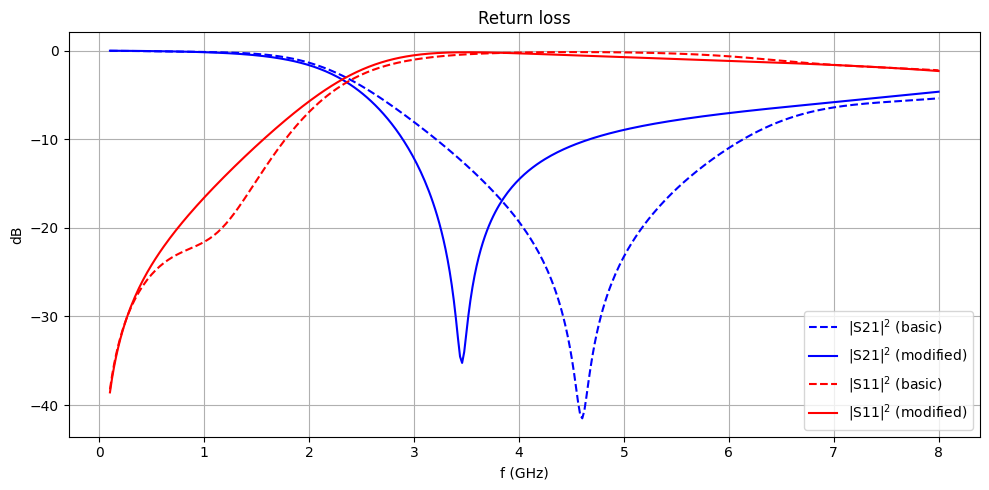
Below, we compare the insertion and return loss of the two resonator designs. Notice that the S21 amplitude falls off much more quickly past 2 GHz in the modified resonator, indicating a sharper filter response.
fig, ax = plt.subplots(figsize=(10, 5), tight_layout=True)
ax.plot(freqs / 1e9, S21dB, "b--", label="|S21|$^2$ (basic)")
ax.plot(freqs / 1e9, S21dB_2, "b", label="|S21|$^2$ (modified)")
ax.plot(freqs / 1e9, S11dB, "r--", label="|S11|$^2$ (basic)")
ax.plot(freqs / 1e9, S11dB_2, "r", label="|S11|$^2$ (modified)")
ax.set_title("Return loss")
ax.set_xlabel("f (GHz)")
ax.set_ylabel("dB")
ax.legend()
ax.grid()
plt.show()
Roll-off rate
We calculate and compare the ROR below.
print(
    f"Calculated ROR \n -- Basic LC resonator: {calculate_ROR(S21dB):.2f} dB/GHz \n -- Modified resonator: {calculate_ROR(S21dB_2):.2f} dB/GHz"
)
Calculated ROR
 -- Basic LC resonator: 13.02 dB/GHz
 -- Modified resonator: 23.98 dB/GHz
The modified resonator shows an almost 2x improvement in ROR compared to the basic design.
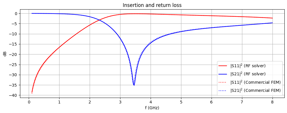
Benchmark Comparison
For benchmarking purposes, we compare the computed S-parameters with results from an independent simulation run on a commercial FEM solver. We find excellent agreement.
# Import benchmark data
freqs_ben, S11dB_ben, S21dB_ben = np.genfromtxt(
    "./misc/wpd-part1-fem.csv", delimiter=",", unpack=True
)
# Plot insertion and return loss
fig, ax = plt.subplots(figsize=(10, 4), tight_layout=True)
ax.plot(freqs / 1e9, S11dB_2, "r", label="|S11|$^2$ (RF solver)")
ax.plot(freqs / 1e9, S21dB_2, "b", label="|S21|$^2$ (RF solver)")
ax.plot(freqs_ben, S11dB_ben, "r:", label="|S11|$^2$ (Commercial FEM)")
ax.plot(freqs_ben, S21dB_ben, "b:", label="|S21|$^2$ (Commercial FEM)")
ax.set_title("Insertion and return loss")
ax.set_xlabel("f (GHz)")
ax.set_ylabel("dB")
ax.legend()
ax.grid()
plt.show()
Conclusion
In this notebook, we compared two different low pass filter designs with the goal of improving ROR performance above 2 GHz. In the next notebook, we will investigate adding a harmonic suppression circuit to improve stopband performance.
Reference
[1] Moloudian, G., Soltani, S., Bahrami, S. et al. Design and fabrication of a Wilkinson power divider with harmonic suppression for LTE and GSM applications. Sci Rep 13, 4246 (2023). https://doi.org/10.1038/s41598-023-31019-7