





Davide Cassara, Harvard John A. Paulson School of Engineering and Applied Sciences
This notebook reproduces the full-wave simulations of the bilayer metalens reported in our paper "Antireflection by design in bilayer metasurfaces", Jaewon Oh, Davide Cassara, Alfonso Palmieri, et al., arXiv:2605.19970 [physics.optics] (2026) (https://arxiv.org/abs/2605.19970).
What we are doing
A conventional single-layer metasurface on glass reflects a few percent of the light at every interface. In the paper we stack two layers of TiO$_2$ nanopillars on top of each other. Each bilayer meta-atom does two jobs at once:
- it imposes the local phase delay needed to shape the wavefront (here, a focusing lens), and
- it acts as a graded impedance-matching stack between air and glass, suppressing reflection.
The notebook simulates the entire 250 µm lens (≈136 000 bilayer pillars, real geometry, no local-phase approximation) and extracts two figures of merit:
- Reflectance of the lens (flux monitor below the device, corrected for the bare-glass area around the lens).
- Focusing efficiency, obtained by propagating the transmitted near field to the focal plane with the angular spectrum method and integrating the power inside a circular iris of diameter 3 × FWHM.
Where we start from: the meta-atom library
The meta-atom library was computed beforehand (RCWA sweeps of the two pillar widths for fixed
layer thicknesses, followed by selection of the (width$_1$, width$_2$) pairs that give full $2\pi$
phase coverage with near-unity transmission). The full derivation of the AR library—how the layer
thicknesses and pillar dimensions are chosen—is described in the paper and its Supplementary
Information; please refer to it for the details. Here we start directly from that library, which is
the file misc/Bilayer Library lambda = 1.31 n = 2.3 U = 0.6 H1 = 0.293 H2 = 1.3.mat:
variable in .mat
|
meaning |
|---|---|
lambda |
design wavelength (µm) — 1.31 µm |
period |
lattice constant $U$ of the square lattice (µm) — 0.6 µm |
nDielectric |
refractive index of the pillars used to build the library — 2.3 |
nSub |
substrate index used to build the library |
d1 |
thickness of layer 1 = top layer (air side) — 0.293 µm |
d2 |
thickness of layer 2 = bottom layer (touches the glass) — 1.3 µm |
radiiLayer1, radiiLayer2
|
pillar size of layer 1 / layer 2 for each library entry (see note below) |
phaseBi, ampBi
|
phase and amplitude of the transmitted field for each library entry |
Square pillars. The pillars are square, not circular. The library keeps the historical
name "radii", and—like the radius of a circle—each value is half the side length of the
square. The pillar width (side) is therefore w = 2 * radii. (You can check this: with
w = 2 r the library phase is reproduced by RCWA and the widths span 0.15–0.54 µm in a 0.6 µm cell.)

Geometry convention used everywhere below (all lengths in µm):
      z
      ^        glass substrate (z > 0, semi-infinite)
      |   ==========================================   z = 0  (glass surface)
      |    ██   ███  ████   ███   ██     layer 2 = bottom, thickness d2, width w2
      |    ▆    ▆▆    ▆▆    ▆▆    ▆      layer 1 = top,    thickness d1, width w1
      |                                   air
      |   ~~~~~~~~~~~~~~ plane wave, x-polarised, travelling +z ~~~~~~~~~~~~~~
Light arrives from air, crosses layer 1 → layer 2 → glass, and focuses inside the substrate.
What you need to provide
Only two numbers: the numerical aperture NA and the lens diameter LENS_DIAMETER_UM.
Everything else (wavelength, lattice constant, pillar heights, index) is read from the library.
If you want a different wavelength, material or lattice, compute a new library with the same
format (see the Appendix at the end) and point LIBRARY_FILE to it—the rest of the notebook
adapts automatically.
Structure of the notebook
- Setup (Sections 0–5) — always run these: inputs, library, phase profile, pillar maps, simulation builders and post-processing tools.
- Part A — nominal lens. One broadband simulation of the lens as designed.
- Part B — top/bottom misalignment sweep. The top layer is shifted laterally by (Δx, Δy).
- Part C — thickness tolerance sweep. The two layer thicknesses are varied independently.
Parts A, B and C are independent of each other: after the setup cells you can run any of them.
Cost. These are large 3D simulations. Every part has a cost-estimate cell and a launch cell guarded by a
RUN_... = Falseflag. Always check the estimate before setting the flag toTrue. A Tidy3D account with an API key is needed (tidy3d configure --apikey=<your key>once in a terminal).
0. Imports
%matplotlib inline

import gc
import json
import time
from pathlib import Path

import numpy as np
import matplotlib.pyplot as plt
import scipy.io as spio
from scipy import fft as sfft

import tidy3d as td
from tidy3d import web

print("Tidy3D version:", td.__version__)
Tidy3D version: 2.12.0
1. User inputs
The only two physical inputs are the numerical aperture and the lens diameter.
The defaults (NA = 0.124, D = 250 µm) correspond to the lens in the paper
(f = 1 mm in air for a 250 µm aperture).
The "advanced" settings below normally don't need to be changed.
# ---------------------------------------------------------------------------
# PHYSICAL INPUTS (the only things you need to choose)
# ---------------------------------------------------------------------------
NA = 0.124                 # numerical aperture of the lens (NA = n * sin(theta_max))
LENS_DIAMETER_UM = 250.0   # lens diameter (µm)

# ---------------------------------------------------------------------------
# ADVANCED SETTINGS
# ---------------------------------------------------------------------------
# Meta-atom library (pre-computed, see the introduction and the paper).
LIBRARY_FILE = Path("misc/Bilayer Library lambda = 1.31 n = 2.3 U = 0.6 H1 = 0.293 H2 = 1.3.mat")

# Tabulated TiO2 refractive index (columns: wavelength in µm, n). Only needed if a
# "dispersive" TiO2 model is selected below.
TIO2_NK_FILE = Path("misc/TiO2_clean.csv")

# Refractive index of the glass substrate used in the full-device simulations.
N_SUBSTRATE = 1.4607

# TiO2 model:  "constant"   -> n = nDielectric from the library (non-dispersive)
#              "dispersive" -> pole-residue fit of TIO2_NK_FILE over the simulated band
TIO2_MODEL_NOMINAL = "dispersive"   # Part A (broadband)
TIO2_MODEL_SWEEPS = "constant"      # Parts B and C (single wavelength)

# Where results are downloaded. Use a folder on a LOCAL disk: cloud-synced folders
# (Google Drive, OneDrive, ...) can cause file-system errors with large HDF5 files.
RESULTS_DIR = Path.home() / "tidy3d_results" / "ar_bilayer_metalens"
RESULTS_DIR.mkdir(parents=True, exist_ok=True)

# Folder name used to group the tasks in the Tidy3D web interface.
TIDY3D_FOLDER = "AR_bilayer_metalens_tutorial"

print("Library file :", LIBRARY_FILE.resolve())
print("Results dir  :", RESULTS_DIR)
Library file : G:\My Drive\Tidy3D Tutorial\Bilayer Library lambda = 1.31 n = 2.3 U = 0.6 H1 = 0.293 H2 = 1.3.mat
Results dir  : C:\Users\Davide Cassara\tidy3d_results\ar_bilayer_metalens
2. Load the meta-atom library
We read the library and convert it to the quantities used in the rest of the notebook.
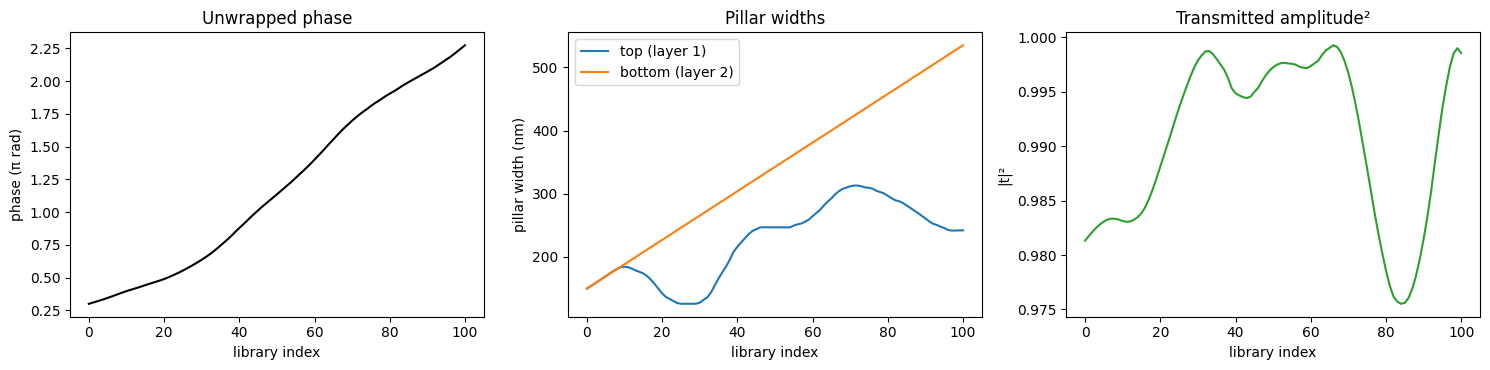
- The phase
phaseBiis stored wrapped to $(-\pi, \pi]$. We unwrap it: the unwrapped phase increases monotonically with the library index and covers almost $2\pi$. This monotonicity is what allows a simple 1D interpolation in Section 4. - The pillar widths are
w = 2 * radii(square pillars, see the introduction).
lib = spio.loadmat(LIBRARY_FILE)

def _scalar(key):
    return float(np.squeeze(lib[key]))

# Design parameters stored in the library
WL0_UM = _scalar("lambda")                         # design wavelength (µm)
PERIOD_XY = np.ravel(lib["period"]).astype(float)  # [Px, Py] (µm)
assert np.isclose(PERIOD_XY[0], PERIOD_XY[-1]), "This notebook assumes a square lattice."
PITCH_UM = float(PERIOD_XY[0])                     # lattice constant U (µm)
H_TOP_UM = _scalar("d1")                           # layer 1 = TOP layer (air side) thickness
H_BOT_UM = _scalar("d2")                           # layer 2 = BOTTOM layer (on glass) thickness
N_TIO2_LIB = _scalar("nDielectric")                # pillar index used for the library
N_SUB_LIB = _scalar("nSub")                        # substrate index used for the library

# Library entries (one row = one bilayer meta-atom)
lib_phase = np.unwrap(np.ravel(lib["phaseBi"]))     # transmitted phase (rad), unwrapped
lib_amp = np.ravel(lib["ampBi"])                    # transmitted amplitude
lib_w_top = 2.0 * np.ravel(lib["radiiLayer1"])      # width of the TOP pillar (µm)
lib_w_bot = 2.0 * np.ravel(lib["radiiLayer2"])      # width of the BOTTOM pillar (µm)
n_lib = lib_phase.size

assert np.all(np.diff(lib_phase) > 0), "Unwrapped library phase must increase monotonically."
phase_coverage = lib_phase[-1] - lib_phase[0]

print(f"Design wavelength       : {WL0_UM:.3f} µm")
print(f"Lattice constant        : {PITCH_UM:.3f} µm")
print(f"Top layer (1) thickness : {H_TOP_UM:.3f} µm   (air side)")
print(f"Bottom layer (2) thick. : {H_BOT_UM:.3f} µm   (touches the glass)")
print(f"Pillar index (library)  : {N_TIO2_LIB:.3f}    substrate index (library): {N_SUB_LIB:.3f}")
print(f"Library entries         : {n_lib}")
print(f"Top widths    : {lib_w_top.min():.3f} – {lib_w_top.max():.3f} µm")
print(f"Bottom widths : {lib_w_bot.min():.3f} – {lib_w_bot.max():.3f} µm")
print(f"Phase coverage: {phase_coverage:.3f} rad  ({phase_coverage / (2*np.pi) * 100:.1f}% of 2π)")
print(f"Amplitude     : {lib_amp.min():.4f} – {lib_amp.max():.4f}")

fig, ax = plt.subplots(1, 3, figsize=(15, 3.8))
idx = np.arange(n_lib)
ax[0].plot(idx, lib_phase / np.pi, "k")
ax[0].set_xlabel("library index"); ax[0].set_ylabel("phase (π rad)"); ax[0].set_title("Unwrapped phase")
ax[1].plot(idx, lib_w_top * 1e3, label="top (layer 1)")
ax[1].plot(idx, lib_w_bot * 1e3, label="bottom (layer 2)")
ax[1].set_xlabel("library index"); ax[1].set_ylabel("pillar width (nm)"); ax[1].legend(); ax[1].set_title("Pillar widths")
ax[2].plot(idx, lib_amp**2, "C2")
ax[2].set_xlabel("library index"); ax[2].set_ylabel("|t|²"); ax[2].set_title("Transmitted amplitude²")
plt.tight_layout(); plt.show()
Design wavelength       : 1.310 µm
Lattice constant        : 0.600 µm
Top layer (1) thickness : 0.293 µm   (air side)
Bottom layer (2) thick. : 1.300 µm   (touches the glass)
Pillar index (library)  : 2.300    substrate index (library): 1.444
Library entries         : 101
Top widths    : 0.126 – 0.313 µm
Bottom widths : 0.150 – 0.535 µm
Phase coverage: 6.205 rad  (98.8% of 2π)
Amplitude     : 0.9877 – 0.9996
3. Target phase profile of the metalens
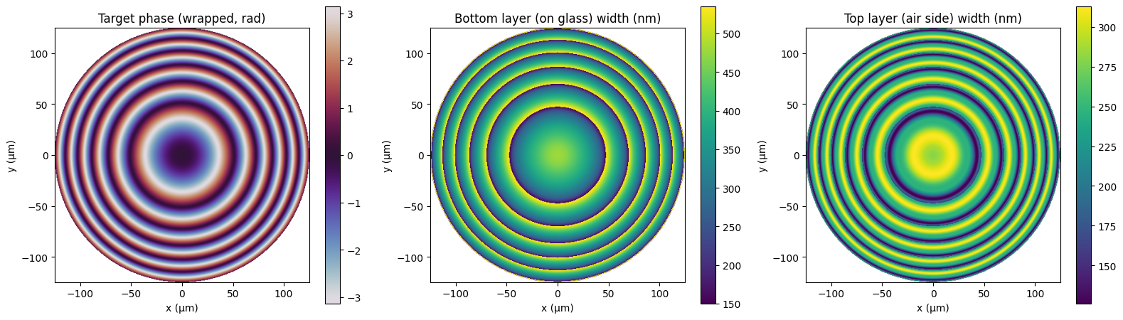
The metalens must convert the incident plane wave into a spherical wave converging to a point at distance $f$ on axis. The phase it must impose at the position $(x, y)$ is the standard hyperbolic ("master") equation
$$ \varphi(x,y) \;=\; -\frac{2\pi\, n_f}{\lambda_0}\left(\sqrt{x^2+y^2+f^2}-f\right), $$
where $n_f$ is the refractive index of the medium in which the light focuses. In the simulation the light exits the lens into (semi-infinite) glass, so the lens focuses inside the substrate, $n_f = n_\text{glass}$. The sign follows Tidy3D's $e^{-i\omega t}$ convention, in which a larger optical path gives a larger phase (as in the library).
The focal length follows from the NA and the lens radius $R = D/2$.
The lens is sampled on the square lattice of the library: one bilayer meta-atom per unit cell, with cell centres placed symmetrically around the origin (this keeps the design mirror-symmetric, which we exploit in Parts A and C to reduce the simulation cost by 4×).
LENS_RADIUS_UM = LENS_DIAMETER_UM / 2
N_FOCUS = N_SUBSTRATE                                   # the lens focuses inside the glass
assert 0 < NA < N_FOCUS, "NA must be smaller than the index of the focusing medium."

theta_max = np.arcsin(NA / N_FOCUS)
FOCAL_LENGTH_UM = LENS_RADIUS_UM / np.tan(theta_max)
print(f"Lens diameter : {LENS_DIAMETER_UM:.1f} µm")
print(f"NA            : {NA:.4f}")
print(f"Focal length  : {FOCAL_LENGTH_UM:.1f} µm  (in glass, n = {N_FOCUS:.4f})")
print(f"  equivalent focal length in air: {LENS_RADIUS_UM / np.tan(np.arcsin(NA)):.1f} µm")
print(f"Diffraction-limited spot (λ/2NA): {WL0_UM / (2 * NA):.2f} µm")

# --- Unit-cell centres: symmetric square grid covering the aperture ---------------
n_pix = int(np.ceil(LENS_DIAMETER_UM / PITCH_UM))
pix_coords = (np.arange(n_pix) - (n_pix - 1) / 2) * PITCH_UM
PX, PY = np.meshgrid(pix_coords, pix_coords, indexing="ij")   # PX[i, j] = x_i, PY[i, j] = y_j
PR = np.hypot(PX, PY)
IN_APERTURE = PR <= LENS_RADIUS_UM                           # pillars only inside the circle

# --- Master equation ---------------------------------------------------------------
def lens_phase(r_um, f_um=FOCAL_LENGTH_UM, wl_um=WL0_UM, n=N_FOCUS):
    # Hyperbolic phase profile of an aberration-free lens focusing a normal plane wave.
    return -2 * np.pi * n / wl_um * (np.sqrt(r_um**2 + f_um**2) - f_um)

PHI_TARGET = lens_phase(PR)

print(f"Unit cells: {n_pix} x {n_pix} = {n_pix**2:,}   |   inside the aperture: {IN_APERTURE.sum():,}")
print(f"Number of 2π zones across the radius: {abs(PHI_TARGET[IN_APERTURE].min()) / (2*np.pi):.1f}")
Lens diameter : 250.0 µm
NA            : 0.1240
Focal length  : 1467.2 µm  (in glass, n = 1.4607)
  equivalent focal length in air: 1000.3 µm
Diffraction-limited spot (λ/2NA): 5.28 µm
Unit cells: 417 x 417 = 173,889   |   inside the aperture: 136,349
Number of 2π zones across the radius: 5.9
4. From phase to pillars: interpolating the library at each lattice site
For each unit cell we need the bilayer meta-atom whose transmitted phase equals the target phase (modulo $2\pi$). Because the unwrapped library phase is monotonic, the procedure is:
- Bring the target phase into the library window: $\varphi_\text{rel} = (\varphi - \varphi_\text{lib,min}) \bmod 2\pi$.
- Find the (fractional) library index whose phase equals $\varphi_\text{rel}$ by linear interpolation.
- Interpolate the top and bottom widths at that fractional index.
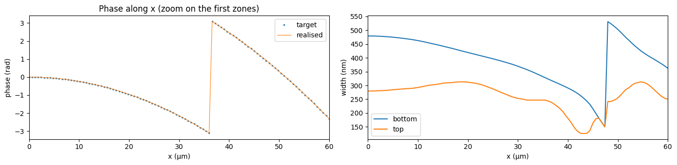
The library covers slightly less than $2\pi$. Target phases that fall in the small uncovered gap are assigned to the closer end of the library. The resulting phase error is plotted below.
(A constant phase offset added to $\varphi$ does not change the lens; it only changes which pillar is used at the centre. We keep it at zero.)
def phase_to_widths(phi_target):
    # Map a target phase (any shape, rad) to (w_top, w_bottom, realised phase, realised amplitude).
    phi0 = lib_phase[0]
    span = lib_phase[-1] - phi0
    phi_rel = np.mod(phi_target - phi0, 2 * np.pi)            # in [0, 2π)

    # Phases inside the uncovered gap (span, 2π): snap to the closest end of the library.
    in_gap = phi_rel > span
    snap_to_end = in_gap & ((phi_rel - span) < (2 * np.pi - phi_rel))
    phi_rel = np.where(in_gap, np.where(snap_to_end, span, 0.0), phi_rel)

    s = np.interp(phi_rel, lib_phase - phi0, np.arange(n_lib))   # fractional library index
    idx = np.arange(n_lib)
    w_top = np.interp(s, idx, lib_w_top)
    w_bot = np.interp(s, idx, lib_w_bot)
    phi_real = np.interp(s, idx, lib_phase)
    amp_real = np.interp(s, idx, lib_amp)
    return w_top, w_bot, phi_real, amp_real

W_TOP, W_BOT, PHI_REAL, AMP_REAL = phase_to_widths(PHI_TARGET)
phase_err = np.angle(np.exp(1j * (PHI_REAL - PHI_TARGET)))

print(f"Top widths used    : {W_TOP[IN_APERTURE].min()*1e3:.1f} – {W_TOP[IN_APERTURE].max()*1e3:.1f} nm")
print(f"Bottom widths used : {W_BOT[IN_APERTURE].min()*1e3:.1f} – {W_BOT[IN_APERTURE].max()*1e3:.1f} nm")
print(f"RMS phase error    : {np.sqrt(np.mean(phase_err[IN_APERTURE]**2)):.4f} rad "
      f"(max {np.abs(phase_err[IN_APERTURE]).max():.4f} rad)")

# --- Plots --------------------------------------------------------------------------
ext = [pix_coords[0], pix_coords[-1], pix_coords[0], pix_coords[-1]]
show = lambda a: np.where(IN_APERTURE, a, np.nan).T          # .T -> imshow rows = y

fig, ax = plt.subplots(1, 3, figsize=(16, 4.6))
im = ax[0].imshow(show(np.angle(np.exp(1j * PHI_TARGET))), origin="lower", extent=ext, cmap="twilight")
ax[0].set_title("Target phase (wrapped, rad)"); plt.colorbar(im, ax=ax[0])
im = ax[1].imshow(show(W_BOT * 1e3), origin="lower", extent=ext, cmap="viridis")
ax[1].set_title("Bottom layer (on glass) width (nm)"); plt.colorbar(im, ax=ax[1])
im = ax[2].imshow(show(W_TOP * 1e3), origin="lower", extent=ext, cmap="viridis")
ax[2].set_title("Top layer (air side) width (nm)"); plt.colorbar(im, ax=ax[2])
for a in ax:
    a.set_xlabel("x (µm)"); a.set_ylabel("y (µm)")
plt.tight_layout(); plt.show()

# Radial cut along +x through the centre
j0 = np.argmin(np.abs(pix_coords))
cut = pix_coords >= 0
fig, ax = plt.subplots(1, 2, figsize=(14, 3.5))
ax[0].plot(pix_coords[cut], np.angle(np.exp(1j * PHI_TARGET[cut, j0])), ".", ms=3, label="target")
ax[0].plot(pix_coords[cut], np.angle(np.exp(1j * PHI_REAL[cut, j0])), "-", lw=0.8, label="realised")
ax[0].set_xlabel("x (µm)"); ax[0].set_ylabel("phase (rad)"); ax[0].legend(); ax[0].set_xlim(0, 60)
ax[0].set_title("Phase along x (zoom on the first zones)")
ax[1].plot(pix_coords[cut], W_BOT[cut, j0] * 1e3, label="bottom")
ax[1].plot(pix_coords[cut], W_TOP[cut, j0] * 1e3, label="top")
ax[1].set_xlabel("x (µm)"); ax[1].set_ylabel("width (nm)"); ax[1].legend(); ax[1].set_xlim(0, 60)
plt.tight_layout(); plt.show()
Top widths used    : 125.9 – 313.0 nm
Bottom widths used : 150.0 – 535.0 nm
RMS phase error    : 0.0025 rad (max 0.0390 rad)
5. Simulation building blocks
This section defines everything shared by Parts A, B and C:
- Materials — glass and TiO$_2$ (constant index or dispersive fit).
-
Nominal geometry — two
GeometryGroups with oneBoxper pillar. They are built once. Sweeps reuse them throughtd.Transformed(a z-scaling for thickness changes, an x/y translation for misalignment), so we never rebuild 136 000 boxes per simulation. -
make_simulation(...)— the complete Tidy3D simulation for a given set of layer heights and top-layer offset. - Post-processing — lens-only reflectance/transmittance and focusing efficiency.
5.1 Materials
SiO2 = td.Medium(permittivity=N_SUBSTRATE**2, name="SiO2")

def make_tio2(model, wl_min_um, wl_max_um):
    # Return the TiO2 medium used for the pillars.
    if model == "constant":
        return td.Medium(permittivity=N_TIO2_LIB**2, name="TiO2")
    if model == "dispersive":
        from tidy3d.plugins.dispersion import FastDispersionFitter, AdvancedFastFitterParam
        fitter = FastDispersionFitter.from_file(str(TIO2_NK_FILE), skiprows=1, delimiter=",")
        fitter = fitter.updated_copy(wvl_range=(wl_min_um, wl_max_um))   # fit only the simulated band
        medium, rms = fitter.fit(max_num_poles=1,
                                 advanced_param=AdvancedFastFitterParam(weights=(1, 1)),
                                 tolerance_rms=2e-5)
        n_fit = np.sqrt(medium.eps_model(td.C_0 / WL0_UM)).real
        print(f"TiO2 dispersive fit: RMS error {rms:.2e}, n({WL0_UM} µm) = {n_fit:.4f}")
        return medium.updated_copy(name="TiO2")
    raise ValueError(f"Unknown TiO2 model: {model!r}")
5.2 Nominal bilayer geometry
Bottom pillars occupy $-d_2 \le z \le 0$ (touching the glass at $z=0$); top pillars sit on them, $-(d_2+d_1) \le z \le -d_2$. Building ≈136 000 boxes per layer takes ~20 s; plotting the full structure (next cells) takes a few minutes because every pillar is drawn.
t0 = time.time()
_xs, _ys = PX[IN_APERTURE], PY[IN_APERTURE]
_wb, _wt = W_BOT[IN_APERTURE], W_TOP[IN_APERTURE]

BOTTOM_NOMINAL = td.GeometryGroup(geometries=[
    td.Box(center=(float(x), float(y), -H_BOT_UM / 2), size=(float(w), float(w), H_BOT_UM))
    for x, y, w in zip(_xs, _ys, _wb)
])
TOP_NOMINAL = td.GeometryGroup(geometries=[
    td.Box(center=(float(x), float(y), -(H_BOT_UM + H_TOP_UM / 2)), size=(float(w), float(w), H_TOP_UM))
    for x, y, w in zip(_xs, _ys, _wt)
])
print(f"Built {len(_wb):,} bottom + {len(_wt):,} top pillars in {time.time() - t0:.1f} s")


def make_bilayer_geometry(h_bot_um=H_BOT_UM, h_top_um=H_TOP_UM, dx_um=0.0, dy_um=0.0):
    # Return (bottom, top) geometries for arbitrary layer heights and a lateral top-layer offset.
    #
    # Bottom layer: scale z by h_bot/h_bot_nom about z = 0 -> it still starts at the glass (z = 0).
    # Top layer   : scale z by h_top/h_top_nom, then translate so that it sits on the new bottom
    #               layer, and shift laterally by (dx, dy) to model an overlay (alignment) error.
    s_b = h_bot_um / H_BOT_UM
    s_t = h_top_um / H_TOP_UM

    bottom = BOTTOM_NOMINAL
    if not np.isclose(s_b, 1.0):
        bottom = td.Transformed(geometry=BOTTOM_NOMINAL, transform=td.Transformed.scaling(1, 1, s_b))

    # After z-scaling the nominal top layer spans [-s_t (Hb+Ht), -s_t Hb]; we want [-(hb+ht), -hb].
    dz = -h_bot_um + s_t * H_BOT_UM
    top = TOP_NOMINAL
    if not (np.isclose(s_t, 1.0) and np.isclose(dz, 0) and dx_um == 0 and dy_um == 0):
        transform = td.Transformed.translation(dx_um, dy_um, dz) @ td.Transformed.scaling(1, 1, s_t)
        top = td.Transformed(geometry=TOP_NOMINAL, transform=transform)
    return bottom, top
Built 136,349 bottom + 136,349 top pillars in 17.7 s
5.3 Simulation factory
- Source — x-polarised plane wave at normal incidence, launched in air just below the pillars and travelling towards $+z$.
- Domain — the lens plus a 5 µm air/glass margin in x and y, PML on all sides. The glass fills $z>0$ and runs into the PML (semi-infinite substrate).
-
Monitors
-
refl— flux plane in air, 1 µm below the pillars (reflected power). -
trans— flux plane in glass, 1 µm above the glass surface (transmitted power). -
nearfield— tangential $E_x, E_y, H_x, H_y$ on the same plane astrans, restricted to the lens aperture, at the design wavelength. This is the field we propagate to the focal plane. It sits 1 µm inside the glass so that evanescent fields have decayed and the plane can be safely down-sampled (interval_space) to keep the files small.
-
-
Symmetry — for an x-polarised normal plane wave and a mirror-symmetric lens,
symmetry=(-1, 1, 0)(PEC-like at x = 0, PMC-like at y = 0) simulates only one quarter of the domain. Tidy3D expands the results back to the full domain, so all monitors are used exactly as without symmetry. A lateral misalignment breaks this symmetry, so Part B runs without it.
PML_BUFFER_UM = 5.0      # lateral margin between lens edge and PML (µm)
SOURCE_GAP_UM = 0.1      # source sits this far below the top of the pillars (µm)
REFL_GAP_UM = 1.0        # reflection monitor this far below the top of the pillars (µm)
Z_NEARFIELD_UM = 1.0     # transmission / near-field plane, inside the glass (µm)
ZMAX_UM = 4.0            # top of the domain (in glass) before the PML (µm)


def make_simulation(*, tio2, freqs, fwidth, h_bot_um=H_BOT_UM, h_top_um=H_TOP_UM,
                    dx_um=0.0, dy_um=0.0, stack_height_max_um=None, min_steps_per_wvl=8,
                    symmetry=(0, 0, 0), nearfield_interval=3, add_xz_monitor=False,
                    run_time_factor=100):
    # stack_height_max_um: tallest stack in a sweep. Source and reflection monitor are placed
    # relative to it, so they stay at the SAME position for every simulation of a sweep.
    h_stack = h_bot_um + h_top_um
    h_ref = h_stack if stack_height_max_um is None else stack_height_max_um
    f0 = td.C_0 / WL0_UM

    z_src = -h_ref - SOURCE_GAP_UM
    z_refl = -h_ref - REFL_GAP_UM
    zmin = min(-4.0, z_refl - 1.5)
    span_xy = LENS_DIAMETER_UM + 2 * PML_BUFFER_UM

    substrate = td.Structure(
        geometry=td.Box(center=(0, 0, (ZMAX_UM + 10) / 2), size=(td.inf, td.inf, ZMAX_UM + 10)),
        medium=SiO2,
    )
    geo_bot, geo_top = make_bilayer_geometry(h_bot_um, h_top_um, dx_um, dy_um)
    pillars_bot = td.Structure(geometry=geo_bot, medium=tio2)
    pillars_top = td.Structure(geometry=geo_top, medium=tio2)

    source = td.PlaneWave(
        source_time=td.GaussianPulse(freq0=f0, fwidth=fwidth),
        size=(td.inf, td.inf, 0),
        center=(0, 0, z_src),
        direction="+",
        pol_angle=0,              # E along x
        name="plane_wave",
    )

    nf_size = LENS_DIAMETER_UM + 4.0
    monitors = [
        td.FluxMonitor(center=(0, 0, z_refl), size=(td.inf, td.inf, 0), freqs=list(freqs), name="refl"),
        td.FluxMonitor(center=(0, 0, Z_NEARFIELD_UM), size=(td.inf, td.inf, 0), freqs=list(freqs), name="trans"),
        td.FieldMonitor(
            center=(0, 0, Z_NEARFIELD_UM), size=(nf_size, nf_size, 0), freqs=[f0],
            fields=["Ex", "Ey", "Hx", "Hy"], interval_space=(nearfield_interval, nearfield_interval, 1),
            colocate=True, name="nearfield",
        ),
    ]
    if add_xz_monitor:   # cross-section of the fields through the pillars (visualisation only)
        monitors.append(td.FieldMonitor(center=(0, 0, 0), size=(td.inf, 0, td.inf), freqs=[f0],
                                        fields=["Ex"], name="xz"))

    return td.Simulation(
        center=(0, 0, (zmin + ZMAX_UM) / 2),
        size=(span_xy, span_xy, ZMAX_UM - zmin),
        grid_spec=td.GridSpec.auto(min_steps_per_wvl=min_steps_per_wvl, wavelength=WL0_UM),
        structures=[substrate, pillars_bot, pillars_top],
        sources=[source],
        monitors=monitors,
        run_time=run_time_factor / fwidth,
        boundary_spec=td.BoundarySpec.all_sides(boundary=td.PML()),
        symmetry=symmetry,
    )


def gaussian_band(bandwidth_um, n_freqs):
    # Source bandwidth (Hz) and monitor frequencies for a band centred at WL0_UM.
    f_lo, f_hi = td.C_0 / (WL0_UM + bandwidth_um / 2), td.C_0 / (WL0_UM - bandwidth_um / 2)
    f0 = td.C_0 / WL0_UM
    freqs = np.array([f0]) if n_freqs == 1 else np.linspace(f_lo, f_hi, n_freqs)
    return freqs, f_hi - f_lo


def plot_structure(sim, title=""):
    # Quick geometry check: x-z cut near the centre and x-y cuts through each layer (zoomed).
    h_b = sim.structures[1].geometry.bounds[1][2] - sim.structures[1].geometry.bounds[0][2]
    z_bot = sim.structures[1].geometry.bounds[0][2]
    z_top_lo, z_top_hi = sim.structures[2].geometry.bounds[0][2], sim.structures[2].geometry.bounds[1][2]
    y_cut = float(pix_coords[np.argmin(np.abs(pix_coords))])   # a row of pillar centres
    fig, ax = plt.subplots(1, 3, figsize=(16, 4.5))
    sim.plot_eps(y=y_cut, ax=ax[0], freq=td.C_0 / WL0_UM)
    ax[0].set_xlim(-6, 6); ax[0].set_ylim(z_top_lo - 1.5, 1.5)
    ax[0].set_title(f"{title}  x–z cut (y = {y_cut:.2f} µm)")
    sim.plot(z=z_bot / 2, ax=ax[1]); ax[1].set_xlim(-6, 6); ax[1].set_ylim(-6, 6)
    ax[1].set_title("bottom layer (z = -d2/2)")
    sim.plot(z=(z_top_lo + z_top_hi) / 2, ax=ax[2]); ax[2].set_xlim(-6, 6); ax[2].set_ylim(-6, 6)
    ax[2].set_title("top layer")
    plt.tight_layout(); plt.show()
5.4 Post-processing: reflectance and transmittance of the lens
Tidy3D normalises the flux to the power injected by the plane wave over the whole $L_x \times L_y$ cross-section of the domain. The lens only covers the fraction $a = \pi R^2 / (L_x L_y)$; the rest is bare glass, whose reflectance is the Fresnel value $R_\text{glass} = \left(\frac{n-1}{n+1}\right)^2$. The lens-only quantities are then
$$ R_\text{lens} = \frac{R_\text{raw} - (1-a)\,R_\text{glass}}{a}, \qquad T_\text{lens} = \frac{T_\text{raw} - (1-a)\,(1-R_\text{glass})}{a}. $$
R_GLASS = ((N_SUBSTRATE - 1) / (N_SUBSTRATE + 1)) ** 2


def lens_area_fraction(sim):
    return np.pi * LENS_RADIUS_UM**2 / (sim.size[0] * sim.size[1])


def lens_only_RT(sim_data):
    # Return lens-only reflectance and transmittance (arrays over the monitor frequencies).
    a = lens_area_fraction(sim_data.simulation)
    R_raw = -np.asarray(sim_data["refl"].flux.values)    # reflected power flows along -z
    T_raw = np.asarray(sim_data["trans"].flux.values)
    R_lens = (R_raw - (1 - a) * R_GLASS) / a
    T_lens = (T_raw - (1 - a) * (1 - R_GLASS)) / a
    return R_lens, T_lens

print(f"Bare-glass Fresnel reflectance: {R_GLASS * 100:.2f}%")
Bare-glass Fresnel reflectance: 3.51%
5.5 Post-processing: focusing efficiency
We compute the focusing efficiency the same way it is defined experimentally: the power that passes through a circular iris of diameter 3 × FWHM centred on the focal spot.
-
Near field. Take $E_x, E_y, H_x, H_y$ from the
nearfieldmonitor (1 µm inside the glass), interpolate them on a uniform grid and keep only the lens aperture ($r \le R$), so that the light passing through the bare glass around the lens is excluded. - Angular spectrum propagation in the homogeneous glass. Each field component satisfies the Helmholtz equation, so it is propagated by a distance $d$ as $$\tilde{E}(k_x,k_y; z+d) = \tilde{E}(k_x,k_y; z)\, e^{i k_z d}, \qquad k_z=\sqrt{(n k_0)^2-k_x^2-k_y^2}.$$ $E_z$ follows from $\nabla\cdot\mathbf E=0$: $\tilde E_z = -(k_x\tilde E_x + k_y\tilde E_y)/k_z$. We use the band-limited transfer function (Matsushima & Shimobaba, Opt. Express 17, 19662 (2009)) and zero-pad the grid to avoid aliasing over the long propagation distance.
- Power through any plane is $P=\tfrac12\iint \mathrm{Re}(E_xH_y^*-E_yH_x^*)\,dx\,dy$, in the same normalised units as the flux monitors.
From this we report:
- $T_\text{ap}$ = power transmitted through the aperture / power incident on the aperture (cross-check with $T_\text{lens}$ above),
- absolute focusing efficiency $\eta_\text{abs}$ = power in the 3×FWHM iris / power incident on the aperture,
- relative focusing efficiency $\eta_\text{rel}$ = power in the 3×FWHM iris / power transmitted through the aperture.
ASM_DX_UM = 0.2          # uniform sampling for the propagation (must be < λ/(2 n_glass) ≈ 0.45 µm)
FOCAL_CROP_UM = 30.0     # half-width of the focal-plane window that is kept (µm)


def nearfield_on_uniform_grid(sim_data, dx_um=ASM_DX_UM):
    # Interpolate the tangential near field on a uniform grid; zero it outside the lens aperture.
    fd = sim_data["nearfield"]
    n_half = int(np.ceil((LENS_RADIUS_UM + 1.0) / dx_um))
    x = dx_um * np.arange(-n_half, n_half + 1)         # symmetric, contains x = 0
    X, Y = np.meshgrid(x, x, indexing="ij")
    aperture = (np.hypot(X, Y) <= LENS_RADIUS_UM)
    comps = {}
    for c in ("Ex", "Ey", "Hx", "Hy"):
        da = getattr(fd, c).isel(f=0, z=0)             # dims (x, y)
        re = da.real.interp(x=x, y=x).values
        im = da.imag.interp(x=x, y=x).values
        comps[c] = np.where(aperture, re + 1j * im, 0).astype(np.complex64)
    return x, comps


def poynting_z(Ex, Ey, Hx, Hy):
    return 0.5 * np.real(Ex * np.conj(Hy) - Ey * np.conj(Hx))


def _asm_setup(n_grid, dx_um, distance_um, n_medium, wl_um, na):
    # Choose a padded FFT size and build the band-limited transfer function inputs.
    # Padded window L must be large enough that the band limit (set by L and d) still
    # passes every angle up to ~1.5x the lens NA.
    lam_m = wl_um / n_medium
    ratio = n_medium / (1.5 * na)
    L_min = 2 * distance_um / np.sqrt(max(ratio**2 - 1, 1e-6))
    n_fft = sfft.next_fast_len(int(min(max(2 * n_grid, np.ceil(L_min / dx_um)), 16384)))
    fx = sfft.fftfreq(n_fft, d=dx_um)                    # spatial frequencies (1/µm)
    L = n_fft * dx_um
    f_lim = 1.0 / (lam_m * np.sqrt((2 * distance_um / L) ** 2 + 1))
    kx = 2 * np.pi * fx
    k = 2 * np.pi / lam_m
    return n_fft, fx, kx, k, f_lim


def propagate_to_plane(x, comps, distance_um, crop_um=FOCAL_CROP_UM,
                       n_medium=N_SUBSTRATE, wl_um=WL0_UM, na=NA):
    # Angular-spectrum propagation of (Ex, Ey, Hx, Hy) over `distance_um` in a homogeneous medium.
    # Returns the cropped coordinates and the fields Ex, Ey, Ez, Hx, Hy at the new plane.
    dx = x[1] - x[0]
    n_grid = x.size
    n_fft, fx, kx, k, f_lim = _asm_setup(n_grid, dx, distance_um, n_medium, wl_um, na)
    KX, KY = kx[:, None], kx[None, :]
    kz = np.sqrt((k**2 - KX**2 - KY**2).astype(np.complex64))
    band = (np.abs(fx)[:, None] <= f_lim) & (np.abs(fx)[None, :] <= f_lim)
    H = np.where(band, np.exp(1j * kz * distance_um), 0).astype(np.complex64)
    kz_safe = np.where(np.abs(kz) > 1e-9, kz, np.inf)

    # x[0] sits at array index 0, so x = 0 is at index i0 of the (periodic) output grid.
    i0 = int(np.argmin(np.abs(x)))
    m = int(round(crop_um / dx))
    idx = (i0 + np.arange(-m, m + 1)) % n_fft               # periodic FFT grid -> wrap indices
    sl = np.ix_(idx, idx)
    x_out = dx * np.arange(-m, m + 1)

    out = {}
    spec = {c: sfft.fft2(comps[c], s=(n_fft, n_fft), workers=-1) for c in ("Ex", "Ey")}
    spec["Ez"] = -(KX * spec["Ex"] + KY * spec["Ey"]) / kz_safe
    for c in ("Ex", "Ey", "Ez"):
        out[c] = sfft.ifft2(spec[c] * H, workers=-1)[sl]
    del spec
    for c in ("Hx", "Hy"):
        out[c] = sfft.ifft2(sfft.fft2(comps[c], s=(n_fft, n_fft), workers=-1) * H, workers=-1)[sl]
    return x_out, out


def axial_profile(x, comps, z_list_um, crop_um=FOCAL_CROP_UM,
                  n_medium=N_SUBSTRATE, wl_um=WL0_UM, na=NA):
    # |E|^2 on the x-z plane (y = 0) for the distances in z_list_um (from the near-field plane).
    # Uses the fact that the y = 0 row of an inverse 2D FFT is a 1D inverse FFT of the sum over ky.
    dx = x[1] - x[0]
    n_fft, fx, kx, k, _ = _asm_setup(x.size, dx, max(z_list_um), n_medium, wl_um, na)
    KX, KY = kx[:, None], kx[None, :]
    kz = np.sqrt((k**2 - KX**2 - KY**2).astype(np.complex64))
    kz_safe = np.where(np.abs(kz) > 1e-9, kz, np.inf)
    L = n_fft * dx
    i0 = int(np.argmin(np.abs(x)))                        # index of x = 0 and of y = 0
    m = int(round(crop_um / dx))
    sl = (i0 + np.arange(-m, m + 1)) % n_fft
    y_phase = np.exp(2j * np.pi * np.arange(n_fft) * i0 / n_fft)[None, :]   # selects row y = 0

    Sx = sfft.fft2(comps["Ex"], s=(n_fft, n_fft), workers=-1)
    Sy = sfft.fft2(comps["Ey"], s=(n_fft, n_fft), workers=-1)
    Sz = -(KX * Sx + KY * Sy) / kz_safe
    I_xz = np.zeros((len(z_list_um), 2 * m + 1))
    for iz, d in enumerate(z_list_um):
        f_lim = 1.0 / ((wl_um / n_medium) * np.sqrt((2 * d / L) ** 2 + 1))
        band = (np.abs(fx)[:, None] <= f_lim) & (np.abs(fx)[None, :] <= f_lim)
        H = np.where(band, np.exp(1j * kz * d), 0) * y_phase / n_fft
        for S in (Sx, Sy, Sz):
            row = sfft.ifft((S * H).sum(axis=1))
            I_xz[iz] += np.abs(row[sl]) ** 2
    return dx * np.arange(-m, m + 1), I_xz


def fwhm_1d(x, y):
    # Full width at half maximum of a single peak (linear interpolation of the crossings).
    y = np.asarray(y); ip = int(np.argmax(y)); half = y[ip] / 2
    il = ip
    while il > 0 and y[il] > half:
        il -= 1
    ir = ip
    while ir < y.size - 1 and y[ir] > half:
        ir += 1
    xl = np.interp(half, [y[il], y[il + 1]], [x[il], x[il + 1]])
    xr = np.interp(half, [y[ir], y[ir - 1]], [x[ir], x[ir - 1]])
    return xr - xl


def focusing_analysis(sim_data, focal_length_um=FOCAL_LENGTH_UM, iris_factor=3.0, return_fields=False):
    # Propagate the near field to the focal plane and compute the focusing efficiencies.
    x, comps = nearfield_on_uniform_grid(sim_data)
    dA = (x[1] - x[0]) ** 2
    P_aperture = poynting_z(comps["Ex"], comps["Ey"], comps["Hx"], comps["Hy"]).sum() * dA
    P_incident = lens_area_fraction(sim_data.simulation)   # plane wave normalised to 1 over the domain

    distance = focal_length_um - Z_NEARFIELD_UM             # f is measured from the glass surface z = 0
    xf, F = propagate_to_plane(x, comps, distance)
    I = np.abs(F["Ex"])**2 + np.abs(F["Ey"])**2 + np.abs(F["Ez"])**2
    Sz = poynting_z(F["Ex"], F["Ey"], F["Hx"], F["Hy"])

    ip, jp = np.unravel_index(np.argmax(I), I.shape)       # peak of the focal spot
    fwhm_x = fwhm_1d(xf, I[:, jp])
    fwhm_y = fwhm_1d(xf, I[ip, :])
    fwhm = 0.5 * (fwhm_x + fwhm_y)
    XF, YF = np.meshgrid(xf, xf, indexing="ij")
    iris = np.hypot(XF - xf[ip], YF - xf[jp]) <= iris_factor * fwhm / 2
    P_spot = Sz[iris].sum() * dA

    res = dict(
        T_aperture=P_aperture / P_incident,
        eta_abs=P_spot / P_incident,
        eta_rel=P_spot / P_aperture,
        fwhm_um=fwhm, fwhm_x_um=fwhm_x, fwhm_y_um=fwhm_y,
        peak_xy_um=(xf[ip], xf[jp]),
    )
    if return_fields:
        res.update(x_nf=x, comps_nf=comps, x_focal=xf, I_focal=I, Sz_focal=Sz, iris=iris)
    return res


def total_cost(cost):
    # Batch.estimate_cost() returns a number or a {task: cost} dict depending on the Tidy3D version.
    return float(sum(cost.values())) if isinstance(cost, dict) else float(cost)


def load_task_ids(path):
    return json.loads(Path(path).read_text())


def save_task_ids(task_ids, path):
    Path(path).write_text(json.dumps(task_ids, indent=1))
    print(f"Saved {len(task_ids)} task id(s) to {path}")
Part A — Nominal lens (broadband)
The lens exactly as designed, simulated over an 80 nm band around 1.31 µm (11 wavelengths for reflection/transmission; the near field is stored at the design wavelength only). TiO$_2$ uses the dispersive fit and the mesh uses 11 steps per wavelength in the highest-index material. Mirror symmetry reduces the cost by a factor of 4.
A_BANDWIDTH_UM = 0.08          # simulated band (µm)
A_N_FREQS = 11                 # wavelengths recorded by the flux monitors
A_MIN_STEPS_PER_WVL = 11       # mesh resolution
A_NEARFIELD_INTERVAL = 4       # down-sampling of the near-field plane (~0.2 µm spacing)
A_SYMMETRY = (-1, 1, 0)

freqs_A, fwidth_A = gaussian_band(A_BANDWIDTH_UM, A_N_FREQS)
lambdas_A = td.C_0 / freqs_A
tio2_A = make_tio2(TIO2_MODEL_NOMINAL, lambdas_A.min(), lambdas_A.max())

sim_A = make_simulation(
    tio2=tio2_A, freqs=freqs_A, fwidth=fwidth_A,
    min_steps_per_wvl=A_MIN_STEPS_PER_WVL, symmetry=A_SYMMETRY,
    nearfield_interval=A_NEARFIELD_INTERVAL, add_xz_monitor=True,
)
print(f"Domain size (µm): {tuple(round(s, 2) for s in sim_A.size)}")
print(f"Yee cells (full domain, before symmetry): {sim_A.num_cells / 1e6:.0f} million")
plot_structure(sim_A, "Nominal")
c:\Programs\MiniConda\envs\general_env\lib\site-packages\rich\live.py:231:
UserWarning: install "ipywidgets" for Jupyter support
  warnings.warn('install "ipywidgets" for Jupyter support')
12:31:33 Eastern Daylight Time WARNING: Unable to fit with weighted RMS error
                               under 'tolerance_rms' of 2e-05
TiO2 dispersive fit: RMS error 3.56e-03, n(1.31 µm) = 2.2637
Domain size (µm): (260.0, 260.0, 8.09)
Yee cells (full domain, before symmetry): 3078 million
# --- Upload and estimate the cost (does not start the simulation) ---
job_A = web.Job(simulation=sim_A, task_name="AR_bilayer_metalens_nominal", folder_name=TIDY3D_FOLDER)
save_task_ids({"nominal": job_A.task_id}, RESULTS_DIR / "task_ids_A.json")
print(f"Estimated cost: {job_A.estimate_cost():.1f} FlexCredits")
# --- Run (set RUN_A = True after checking the estimate) ---
RUN_A = False
DATA_A = RESULTS_DIR / "nominal.hdf5"

if RUN_A:
    sim_data_A = job_A.run(path=str(DATA_A))
elif DATA_A.exists():
    sim_data_A = td.SimulationData.from_file(str(DATA_A))            # already downloaded
elif (RESULTS_DIR / "task_ids_A.json").exists():                       # finished on the server earlier
    sim_data_A = web.load(load_task_ids(RESULTS_DIR / "task_ids_A.json")["nominal"], path=str(DATA_A))
else:
    sim_data_A = None
    print("No results yet: set RUN_A = True to run the simulation.")
# --- A1. Reflectance and transmittance spectra ---
R_A, T_A = lens_only_RT(sim_data_A)
i_f0 = int(np.argmin(np.abs(lambdas_A - WL0_UM)))
print(f"At λ = {lambdas_A[i_f0]:.3f} µm:  R_lens = {R_A[i_f0]*100:.2f}%   T_lens = {T_A[i_f0]*100:.2f}%   "
      f"(bare glass R = {R_GLASS*100:.2f}%)")

fig, ax = plt.subplots(1, 2, figsize=(12, 3.8))
ax[0].plot(lambdas_A * 1e3, R_A * 100, "o-", label="bilayer lens")
ax[0].axhline(R_GLASS * 100, color="gray", ls="--", label="bare glass")
ax[0].set_xlabel("wavelength (nm)"); ax[0].set_ylabel("reflectance (%)"); ax[0].legend()
ax[1].plot(lambdas_A * 1e3, T_A * 100, "o-", label="T (flux monitor)")
ax[1].plot(lambdas_A * 1e3, (1 - R_A) * 100, "--", label="1 − R")
ax[1].set_xlabel("wavelength (nm)"); ax[1].set_ylabel("transmittance (%)"); ax[1].legend()
plt.tight_layout(); plt.show()
# --- A2. Fields through the pillars and near-field phase ---
sim_data_A.plot_field("xz", "Ex", val="real", eps_alpha=0.3)
plt.xlim(-10, 10); plt.show()

nf_Ex = sim_data_A["nearfield"].Ex.isel(f=0, z=0)
sel = nf_Ex.sel(x=slice(-30, 30), y=slice(-30, 30))
fig, ax = plt.subplots(figsize=(6, 5))
im = ax.pcolormesh(sel.x, sel.y, np.angle(sel.values).T, cmap="twilight", shading="auto")
ax.set_aspect("equal"); ax.set_xlabel("x (µm)"); ax.set_ylabel("y (µm)")
ax.set_title("Phase of Ex, 1 µm inside the glass (centre of the lens)")
plt.colorbar(im, ax=ax); plt.show()
# --- A3. Focusing efficiency ---
foc_A = focusing_analysis(sim_data_A, return_fields=True)
print(f"Transmission through the aperture T_ap : {foc_A['T_aperture']*100:.2f}%  "
      f"(flux-monitor T_lens at λ0: {T_A[i_f0]*100:.2f}%)")
print(f"Focal spot FWHM                        : {foc_A['fwhm_um']:.2f} µm "
      f"(x {foc_A['fwhm_x_um']:.2f}, y {foc_A['fwhm_y_um']:.2f}; Airy {0.514*WL0_UM/NA:.2f} µm)")
print(f"Absolute focusing efficiency η_abs     : {foc_A['eta_abs']*100:.2f}%")
print(f"Relative focusing efficiency η_rel     : {foc_A['eta_rel']*100:.2f}%")

xf, I = foc_A["x_focal"], foc_A["I_focal"]
fig, ax = plt.subplots(1, 2, figsize=(13, 4.5))
im = ax[0].imshow(I.T / I.max(), origin="lower", extent=[xf[0], xf[-1], xf[0], xf[-1]], cmap="inferno")
r_iris = 1.5 * foc_A["fwhm_um"]
ax[0].add_patch(plt.Circle(foc_A["peak_xy_um"], r_iris, fill=False, color="c", ls="--", label="3×FWHM iris"))
ax[0].set_xlim(-15, 15); ax[0].set_ylim(-15, 15); ax[0].legend(loc="upper right")
ax[0].set_xlabel("x (µm)"); ax[0].set_ylabel("y (µm)"); ax[0].set_title(f"|E|² at the focal plane (z = f = {FOCAL_LENGTH_UM:.0f} µm)")
plt.colorbar(im, ax=ax[0])
ic = I.shape[1] // 2
ax[1].plot(xf, I[:, ic] / I.max(), label="x cut")
ax[1].plot(xf, I[ic, :] / I.max(), "--", label="y cut")
ax[1].axvspan(-r_iris, r_iris, color="c", alpha=0.15, label="iris")
ax[1].set_xlim(-20, 20); ax[1].set_xlabel("position (µm)"); ax[1].set_ylabel("normalised |E|²"); ax[1].legend()
plt.tight_layout(); plt.show()
# --- A4. Optional: intensity along the optical axis (x–z plane, y = 0) ---
z_axis = np.linspace(0.6, 1.4, 81) * FOCAL_LENGTH_UM - Z_NEARFIELD_UM
x_ax, I_xz = axial_profile(foc_A["x_nf"], foc_A["comps_nf"], z_axis)
z_plot = z_axis + Z_NEARFIELD_UM
fig, ax = plt.subplots(1, 2, figsize=(13, 4))
ax[0].imshow(I_xz.T / I_xz.max(), origin="lower", aspect="auto", cmap="inferno",
             extent=[z_plot[0], z_plot[-1], x_ax[0], x_ax[-1]])
ax[0].axvline(FOCAL_LENGTH_UM, color="c", ls="--", lw=0.8)
ax[0].set_xlabel("z (µm)"); ax[0].set_ylabel("x (µm)"); ax[0].set_ylim(-15, 15); ax[0].set_title("|E|², y = 0")
ax[1].plot(z_plot, I_xz[:, I_xz.shape[1] // 2] / I_xz.max())
ax[1].axvline(FOCAL_LENGTH_UM, color="gray", ls="--", label="design f")
ax[1].set_xlabel("z (µm)"); ax[1].set_ylabel("on-axis |E|² (norm.)"); ax[1].legend()
plt.tight_layout(); plt.show()
print(f"On-axis intensity maximum at z = {z_plot[np.argmax(I_xz[:, I_xz.shape[1] // 2])]:.0f} µm "
      f"(design f = {FOCAL_LENGTH_UM:.0f} µm)")
# Note: for lenses with a small Fresnel number R²/(λ f / n) the on-axis maximum sits slightly
# before the geometric focus (the well-known "focal shift"); an ideal lens shows the same shift.
# The focusing efficiency is always evaluated at the design focal plane z = f.
# --- A5. Save the results ---
out = RESULTS_DIR / "AR_bilayer_nominal_results.mat"
spio.savemat(out, {
    "lambda0_um": WL0_UM, "NA": NA, "diameter_um": LENS_DIAMETER_UM, "focal_length_um": FOCAL_LENGTH_UM,
    "lambdas_um": lambdas_A, "R_lens": R_A, "T_lens": T_A, "n_sub": N_SUBSTRATE,
    "T_aperture": foc_A["T_aperture"], "eta_abs": foc_A["eta_abs"], "eta_rel": foc_A["eta_rel"],
    "fwhm_um": foc_A["fwhm_um"], "x_focal_um": foc_A["x_focal"], "I_focal": foc_A["I_focal"],
})
print("Saved:", out)
Part B — Misalignment (overlay) sweep of the top layer
The two layers are defined in separate lithography steps, so the top layer can be shifted with respect to the bottom one. Here the whole top layer is translated by $(\Delta x, \Delta y)$ and we record reflectance and focusing efficiency at the design wavelength.
- Offsets from 0 to 260 nm in 26 nm steps along x and y (11 × 11 = 121 simulations). Negative offsets follow from the mirror symmetry of the lens, so only one quadrant is needed.
- Single wavelength (narrow-band pulse), constant-index TiO$_2$ (as in the library), 8 mesh steps per wavelength.
- No symmetry: a lateral offset breaks the mirror symmetry of the structure.
Building the 121 simulation objects takes a few minutes on a laptop (the geometry is shared, not copied).
⚠️ Cost: 121 full-device simulations. For a first test, use a coarser grid (e.g.
B_OFFSET_STEP_NM = 130, 9 simulations).
B_OFFSET_STEP_NM = 26
B_OFFSET_MAX_NM = 260
B_MIN_STEPS_PER_WVL = 8
B_NEARFIELD_INTERVAL = 3
B_SOURCE_BANDWIDTH_UM = 0.05

offsets_nm = np.arange(0, B_OFFSET_MAX_NM + B_OFFSET_STEP_NM / 2, B_OFFSET_STEP_NM)
N_B = offsets_nm.size
freqs_B, fwidth_B = gaussian_band(B_SOURCE_BANDWIDTH_UM, 1)
tio2_B = make_tio2(TIO2_MODEL_SWEEPS, WL0_UM - 0.02, WL0_UM + 0.02)

def key_B(dx_nm, dy_nm):
    return f"dx{int(round(dx_nm)):03d}_dy{int(round(dy_nm)):03d}"

sims_B = {}
t0 = time.time()
for dx_nm in offsets_nm:
    for dy_nm in offsets_nm:
        sims_B[key_B(dx_nm, dy_nm)] = make_simulation(
            tio2=tio2_B, freqs=freqs_B, fwidth=fwidth_B,
            dx_um=dx_nm / 1e3, dy_um=dy_nm / 1e3,
            min_steps_per_wvl=B_MIN_STEPS_PER_WVL, symmetry=(0, 0, 0),
            nearfield_interval=B_NEARFIELD_INTERVAL,
        )
print(f"Built {len(sims_B)} simulations in {time.time() - t0:.0f} s  |  offsets (nm): {offsets_nm.astype(int).tolist()}")
plot_structure(sims_B[key_B(offsets_nm[-1], offsets_nm[-1])], f"Δx = Δy = {offsets_nm[-1]:.0f} nm")
# --- Upload and estimate the cost (does not start the simulations) ---
batch_B = web.Batch(simulations=sims_B, folder_name=TIDY3D_FOLDER, verbose=True)
batch_B.upload()
save_task_ids({k: job.task_id for k, job in batch_B.jobs.items()}, RESULTS_DIR / "task_ids_B.json")
print(f"Estimated cost: {total_cost(batch_B.estimate_cost()):.1f} FlexCredits for {len(sims_B)} simulations")
# --- Run (set RUN_B = True after checking the estimate) ---
RUN_B = False
if RUN_B:
    batch_B.start()
    batch_B.monitor()
else:
    print("Not started. Set RUN_B = True to launch the sweep.")
Analysis. Results are downloaded one at a time (skipped if already on disk), reduced to a few
numbers and released from memory, so the loop also works after a kernel restart: re-run the setup
cells (0–5) and the first cell of this part (to define offsets_nm), then run the cell below.
task_ids_B = load_task_ids(RESULTS_DIR / "task_ids_B.json")
dir_B = RESULTS_DIR / "misalignment"; dir_B.mkdir(exist_ok=True)

R_B = np.full((N_B, N_B), np.nan)          # axis 0: Δx, axis 1: Δy
T_B = np.full((N_B, N_B), np.nan)
ETA_ABS_B = np.full((N_B, N_B), np.nan)
ETA_REL_B = np.full((N_B, N_B), np.nan)

for i, dx_nm in enumerate(offsets_nm):
    for j, dy_nm in enumerate(offsets_nm):
        key = key_B(dx_nm, dy_nm)
        try:
            sd = web.load(task_ids_B[key], path=str(dir_B / f"{key}.hdf5"), replace_existing=False, verbose=False)
        except Exception as exc:
            print(f"skip {key}: {exc}")
            continue
        R, T = lens_only_RT(sd)
        R_B[i, j], T_B[i, j] = R[0], T[0]
        foc = focusing_analysis(sd)
        ETA_ABS_B[i, j], ETA_REL_B[i, j] = foc["eta_abs"], foc["eta_rel"]
        print(f"{key}: R = {R_B[i, j]*100:.3f}%   η_abs = {ETA_ABS_B[i, j]*100:.2f}%   η_rel = {ETA_REL_B[i, j]*100:.2f}%")
        del sd, foc
        gc.collect()
# --- Heatmaps: change with respect to perfect alignment ---
step = offsets_nm[1] - offsets_nm[0] if N_B > 1 else 1
ext = [offsets_nm[0] - step / 2, offsets_nm[-1] + step / 2, offsets_nm[0] - step / 2, offsets_nm[-1] + step / 2]
dR_B = (R_B - R_B[0, 0]) * 100
dEta_B = (ETA_ABS_B - ETA_ABS_B[0, 0]) * 100
print(f"Perfect alignment: R = {R_B[0,0]*100:.3f}%, η_abs = {ETA_ABS_B[0,0]*100:.2f}%, η_rel = {ETA_REL_B[0,0]*100:.2f}%")

fig, ax = plt.subplots(1, 2, figsize=(13, 5))
for a, data, label, cmap in [(ax[0], dR_B, "ΔR (percentage points)", "hot"),
                             (ax[1], dEta_B, "Δη_abs (percentage points)", "viridis")]:
    im = a.imshow(data.T, origin="lower", extent=ext, cmap=cmap, aspect="equal")
    a.set_xlabel("Δx (nm)"); a.set_ylabel("Δy (nm)")
    plt.colorbar(im, ax=a, label=label)
ax[0].set_title("Reflectance change vs. misalignment"); ax[1].set_title("Focusing-efficiency change vs. misalignment")
plt.tight_layout(); plt.show()

out = RESULTS_DIR / "AR_bilayer_misalignment_sweep.mat"
spio.savemat(out, {"lambda0_um": WL0_UM, "offsets_nm": offsets_nm, "R": R_B, "T": T_B,
                   "eta_abs": ETA_ABS_B, "eta_rel": ETA_REL_B, "n_sub": N_SUBSTRATE,
                   "NA": NA, "diameter_um": LENS_DIAMETER_UM})
print("Saved:", out)
Part C — Thickness tolerance sweep
The thicknesses of the two TiO$_2$ layers are varied independently by ±10% around the nominal values $d_2$ (bottom) and $d_1$ (top), with 11 points each (121 simulations). The pillar widths are kept at their design values. The bottom layer always starts at the glass surface and the top layer always sits on the bottom one.
- Single wavelength, constant-index TiO$_2$, 8 mesh steps per wavelength.
- The structure stays mirror-symmetric, so quarter-domain symmetry is used (4× cheaper).
- Source and reflection monitor are placed with respect to the tallest stack of the sweep, so they are at the same position in every simulation.
Building the simulation objects takes a few minutes.
⚠️ Cost: 121 simulations. Start with e.g.
N_BOTTOM = N_TOP = 3.
BOTTOM_TOL_FRAC = 0.10
TOP_TOL_FRAC = 0.10
N_BOTTOM = 11
N_TOP = 11
C_MIN_STEPS_PER_WVL = 8
C_NEARFIELD_INTERVAL = 3
C_SOURCE_BANDWIDTH_UM = 0.05
C_SYMMETRY = (-1, 1, 0)

bottom_err_nm = np.linspace(-BOTTOM_TOL_FRAC, BOTTOM_TOL_FRAC, N_BOTTOM) * H_BOT_UM * 1e3
top_err_nm = np.linspace(-TOP_TOL_FRAC, TOP_TOL_FRAC, N_TOP) * H_TOP_UM * 1e3
h_bot_list = H_BOT_UM + bottom_err_nm / 1e3
h_top_list = H_TOP_UM + top_err_nm / 1e3
h_stack_max = h_bot_list.max() + h_top_list.max()

freqs_C, fwidth_C = gaussian_band(C_SOURCE_BANDWIDTH_UM, 1)
tio2_C = make_tio2(TIO2_MODEL_SWEEPS, WL0_UM - 0.02, WL0_UM + 0.02)

def key_C(ib, it):
    return f"ib{ib:02d}_it{it:02d}"

sims_C = {}
t0 = time.time()
for ib, hb in enumerate(h_bot_list):
    for it, ht in enumerate(h_top_list):
        sims_C[key_C(ib, it)] = make_simulation(
            tio2=tio2_C, freqs=freqs_C, fwidth=fwidth_C,
            h_bot_um=float(hb), h_top_um=float(ht), stack_height_max_um=h_stack_max,
            min_steps_per_wvl=C_MIN_STEPS_PER_WVL, symmetry=C_SYMMETRY,
            nearfield_interval=C_NEARFIELD_INTERVAL,
        )
i_nom_b = int(np.argmin(np.abs(bottom_err_nm)))
i_nom_t = int(np.argmin(np.abs(top_err_nm)))
print(f"Built {len(sims_C)} simulations in {time.time() - t0:.0f} s")
print(f"Bottom (d2): {h_bot_list[0]*1e3:.1f} – {h_bot_list[-1]*1e3:.1f} nm   |   Top (d1): {h_top_list[0]*1e3:.1f} – {h_top_list[-1]*1e3:.1f} nm")
plot_structure(sims_C[key_C(N_BOTTOM - 1, N_TOP - 1)], "Thickest stack")
# --- Upload and estimate the cost (does not start the simulations) ---
batch_C = web.Batch(simulations=sims_C, folder_name=TIDY3D_FOLDER, verbose=True)
batch_C.upload()
save_task_ids({k: job.task_id for k, job in batch_C.jobs.items()}, RESULTS_DIR / "task_ids_C.json")
print(f"Estimated cost: {total_cost(batch_C.estimate_cost()):.1f} FlexCredits for {len(sims_C)} simulations")
# --- Run (set RUN_C = True after checking the estimate) ---
RUN_C = False
if RUN_C:
    batch_C.start()
    batch_C.monitor()
else:
    print("Not started. Set RUN_C = True to launch the sweep.")
# --- Analysis (works after a kernel restart: re-run setup cells and the first cell of Part C) ---
task_ids_C = load_task_ids(RESULTS_DIR / "task_ids_C.json")
dir_C = RESULTS_DIR / "thickness"; dir_C.mkdir(exist_ok=True)

R_C = np.full((N_BOTTOM, N_TOP), np.nan)
T_C = np.full((N_BOTTOM, N_TOP), np.nan)
ETA_ABS_C = np.full((N_BOTTOM, N_TOP), np.nan)
ETA_REL_C = np.full((N_BOTTOM, N_TOP), np.nan)

for ib in range(N_BOTTOM):
    for it in range(N_TOP):
        key = key_C(ib, it)
        try:
            sd = web.load(task_ids_C[key], path=str(dir_C / f"{key}.hdf5"), replace_existing=False, verbose=False)
        except Exception as exc:
            print(f"skip {key}: {exc}")
            continue
        R, T = lens_only_RT(sd)
        R_C[ib, it], T_C[ib, it] = R[0], T[0]
        foc = focusing_analysis(sd)
        ETA_ABS_C[ib, it], ETA_REL_C[ib, it] = foc["eta_abs"], foc["eta_rel"]
        print(f"{key}: R = {R_C[ib, it]*100:.3f}%   η_abs = {ETA_ABS_C[ib, it]*100:.2f}%   η_rel = {ETA_REL_C[ib, it]*100:.2f}%")
        del sd, foc
        gc.collect()
# --- Heatmaps: change with respect to the nominal thicknesses ---
db = np.diff(bottom_err_nm).mean() if N_BOTTOM > 1 else 1
dt = np.diff(top_err_nm).mean() if N_TOP > 1 else 1
ext = [bottom_err_nm[0] - db / 2, bottom_err_nm[-1] + db / 2, top_err_nm[0] - dt / 2, top_err_nm[-1] + dt / 2]
dR_C = (R_C - R_C[i_nom_b, i_nom_t]) * 100
dEta_C = (ETA_ABS_C - ETA_ABS_C[i_nom_b, i_nom_t]) * 100
print(f"Nominal: R = {R_C[i_nom_b, i_nom_t]*100:.3f}%, η_abs = {ETA_ABS_C[i_nom_b, i_nom_t]*100:.2f}%")

fig, ax = plt.subplots(1, 2, figsize=(13, 5))
for a, data, label, cmap in [(ax[0], dR_C, "ΔR (percentage points)", "hot"),
                             (ax[1], dEta_C, "Δη_abs (percentage points)", "viridis")]:
    im = a.imshow(data.T, origin="lower", extent=ext, cmap=cmap, aspect="auto")
    a.axvline(0, color="w", lw=0.6); a.axhline(0, color="w", lw=0.6)
    a.set_xlabel("bottom-layer (d2) thickness error (nm)"); a.set_ylabel("top-layer (d1) thickness error (nm)")
    a.set_box_aspect(1)
    plt.colorbar(im, ax=a, label=label)
ax[0].set_title("Reflectance change"); ax[1].set_title("Focusing-efficiency change")
plt.tight_layout(); plt.show()

out = RESULTS_DIR / "AR_bilayer_thickness_sweep.mat"
spio.savemat(out, {"lambda0_um": WL0_UM, "bottom_error_nm": bottom_err_nm, "top_error_nm": top_err_nm,
                   "bottom_heights_um": h_bot_list, "top_heights_um": h_top_list,
                   "R": R_C, "T": T_C, "eta_abs": ETA_ABS_C, "eta_rel": ETA_REL_C,
                   "n_sub": N_SUBSTRATE, "NA": NA, "diameter_um": LENS_DIAMETER_UM})
print("Saved:", out)
Appendix — Using your own library
Everything downstream of Section 2 is driven by the library file. To design a lens for a different wavelength, material, lattice constant or pair of layer thicknesses:
- Compute a new bilayer library (e.g. with RCWA), following the procedure in the paper/SI: fix $d_1$, $d_2$ and the lattice constant, sweep the two pillar widths, and select a 1D path of (width$_1$, width$_2$) pairs with high transmission, low reflection and a monotonic phase that covers ~$2\pi$.
- Save it as a
.matfile with the same variables:lambda,period,nDielectric,nSub,d1(top),d2(bottom, on the substrate),radiiLayer1,radiiLayer2(half-side of the square pillars),phaseBi,ampBi. - Set
LIBRARY_FILEin Section 1 (and, if needed,N_SUBSTRATEand the TiO$_2$ model / n,k file).
Things to keep in mind:
- The simulated band, the mesh (
GridSpec.autois set relative tolambda) and the ASM sampling (ASM_DX_UM< λ / (2 n_glass)) all scale with the wavelength automatically, but check them if you move far from 1.31 µm. - The run time, cost and file size scale roughly with (D / λ)² × (thickness / λ). For larger lenses, start with a small diameter to validate the pipeline.
- If your pillars are circular, replace
td.Boxwithtd.Cylinder(axis = 2) in Section 5.2.


 TERMS & CONDITIONS


 How the process works:
 Try this real URL to see an example: