Author: Sumukh Vaidya, Purdue University
In this notebook, we replicate the results of the paper Fiber-Integrated van der Waals Quantum Sensor with an Optimal Cavity Interface .
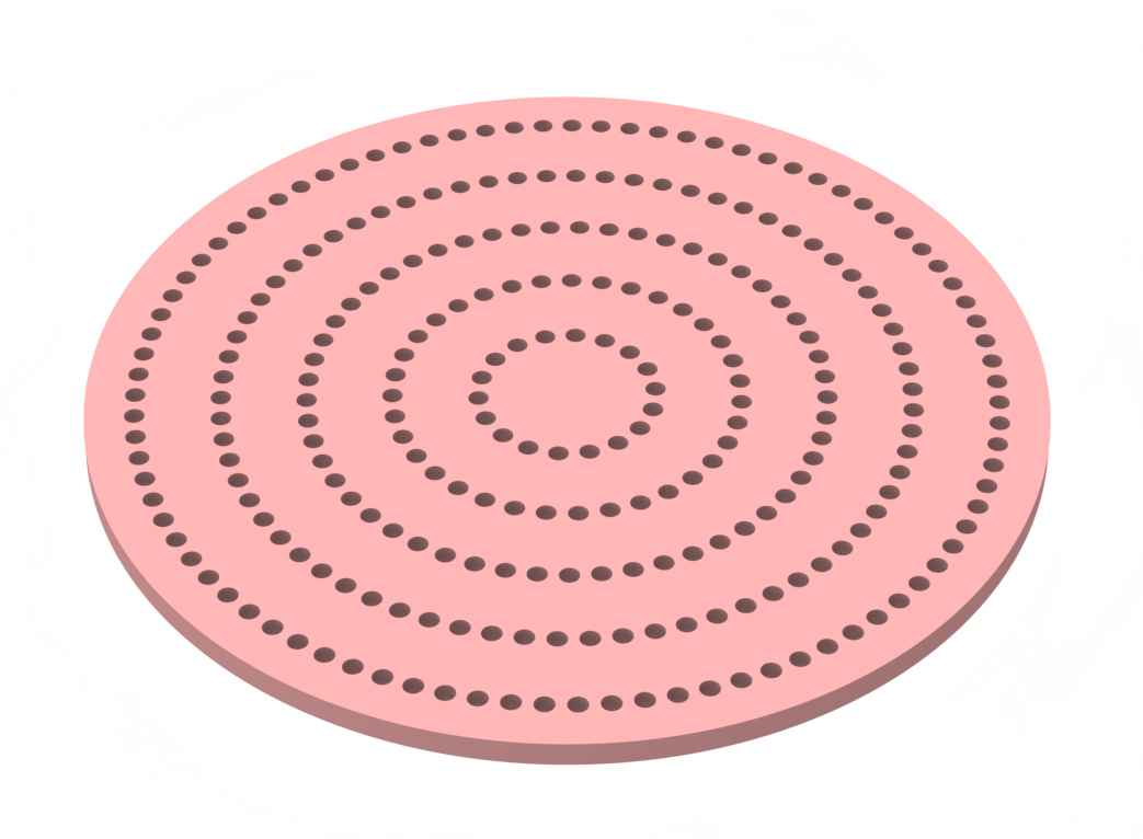
The authors integrate hexagonal Boron Nitride (hBN) into a optic fiber and create a circular Bragg Grating on the hBN. hBN hosts spin defect emitters, which, when coupled with the fiber, can sense magnetic fields.
For this calculation, we will use a point dipole emitting a broadband pulse and monitor the field, and flux inside the optic fiber.
The main idea is to optimally couple the dipole emission into the fiber, so that defect excitation and readout can be done efficiently. The reason to avoid the simple circular Bragg grating design is to maintain the structure when the 2D material is transferred onto a fiber tip.
Another consideration for optimal coupling is the numerical aperture of the fiber. Typical NA for fibers are between 0.1- 0.4. This restricts how much signal from an emitter can be coupled. If the design can improve the amount of flux into a small solid angle along the axis of the fiber, it will have a better signal collection efficiency.
Set Up the Simulation
import numpy as np
import matplotlib.pyplot as plt
import matplotlib.patches as mpatches

import tidy3d as td
from tidy3d.plugins.mode import ModeSolver
from tidy3d import web
# Define structure related parameters
sim_size = [20, 20, 8.5]
sim_x = sim_size[0]
sim_y = sim_size[1]
sim_z = sim_size[2]
grid_spec = td.GridSpec(wavelength=0.85)

lambda0 = 0.85
lambda_low = 0.75
lambda_high = 0.95
npoints = 200
freq0 = td.C_0 / lambda0
fwidth = td.C_0 * (1 / lambda_low - 1 / lambda_high)
freqs = np.linspace(freq0 - fwidth / 2, freq0 + fwidth / 2, npoints)
run_time = 20 / fwidth

r = 0.498  # Radial increment
R0 = 0.645  # Initial inner radius
l = 0.224  # Arc length between holes
a = 0.075  # Hole radius
n_rings = 12  # Number of rings
t_hbn = 0.2  # hBN thickness
center = [0, 0]  # Center of the hole array
# Define the media
Vacuum = td.Medium(
    name="Vacuum",
)

Glass = td.Medium(
    name="Glass",
    permittivity=2.25,
)

mat_hbn = td.Medium.from_nk(n=2.1, k=0, freq=freq0, name="hbn")


# Define the source, a single oscillating point dipole
pointdipole_0 = td.PointDipole(
    name="pointdipole_0",
    source_time=td.GaussianPulse(freq0=freq0, fwidth=fwidth),
    polarization="Ey",
)


# Define the monitors
fluxmonitor_0 = td.FluxMonitor(
    name="fluxmonitor_0",
    size=[0, sim_y, sim_z],
    freqs=freqs,
)

fluxmonitor_1 = td.FluxMonitor(
    name="fluxmonitor_1",
    center=[0, 0, 3],
    size=[sim_x, sim_y, 0],
    freqs=freqs,
)

fluxmonitor_2 = td.FluxMonitor(
    name="fluxmonitor_2",
    center=[0, 0, -3],
    size=[sim_x, sim_y, 0],
    freqs=freqs,
)

fluxmonitor_3 = td.FluxMonitor(
    name="fluxmonitor_3",
    size=[sim_x, 0, sim_z],
    freqs=freqs,
)

fieldmonitor_4 = td.FieldMonitor(
    name="fieldmonitor_4",
    size=[0, sim_y, sim_z],
    freqs=freqs,
)

fieldmonitor_5 = td.FieldMonitor(
    name="fieldmonitor_5",
    size=[sim_x, 0, sim_z],
    freqs=freqs,
)

fieldmonitor_6 = td.FieldMonitor(
    name="fieldmonitor_6",
    center=[0, 0, 3],
    size=[sim_x, sim_y, 0],
    freqs=freqs,
)

fieldmonitor_7 = td.FieldMonitor(
    name="fieldmonitor_7",
    center=[0, 0, -3],
    size=[sim_x, sim_y, 0],
    freqs=freqs,
)

fieldmonitor_8 = td.FieldMonitor(
    name="fieldmonitor_8",
    center=[0, 0, -2],
    size=[sim_x, sim_y, 0],
    freqs=freqs,
)

fieldmonitor_9 = td.FieldMonitor(
    name="fieldmonitor_9",
    center=[0, 0, -1],
    size=[sim_x, sim_y, 0],
    freqs=freqs,
)

fieldmonitor_10 = td.FieldMonitor(
    name="fieldmonitor_10",
    center=[0, 0, -0.2],
    size=[sim_x, sim_y, 0],
    freqs=freqs,
)


# Define the structures

# Glass cylinder, representing optic fiber
cylinder_glass = td.Structure(
    geometry=td.Cylinder(radius=50, center=[0, 0, -2.55], length=4.9),
    name="cylinder_glass",
    medium=Glass,
)

# hBN slab with no holes
cylinder_hbn = td.Structure(
    geometry=td.Cylinder(
        center=[0, 0, 0], radius=R0 + r * (n_rings + 1), length=t_hbn, axis=2
    ),
    medium=mat_hbn,
)


# Function to generate the holes filled with air
def generate_object_0(center, r, R0, l, a, n_rings, t_hbn):
    hole_positions = []
    radii = np.linspace(R0, R0 + r * n_rings, n_rings)
    for R in radii:
        n_angles = int(2 * np.pi * R / l)
        for i in range(n_angles):
            angle = i * 2 * np.pi / n_angles
            x = center[0] + R * np.cos(angle)
            y = center[1] + R * np.sin(angle)
            hole_positions.append([x, y])

    mat_air = td.Medium(permittivity=1, name="air")
    mat_hbn = td.Medium(permittivity=5.1, name="hbn")

    structures = []

    for pos in hole_positions:
        structures.append(
            td.Structure(
                geometry=td.Cylinder(
                    center=[pos[0], pos[1], 0], radius=a, length=t_hbn, axis=2
                ),
                medium=mat_air,
            )
        )

    return structures


generate_object_0_result = generate_object_0(center, r, R0, l, a, n_rings, t_hbn)
generate_object_0_result = (
    generate_object_0_result
    if isinstance(generate_object_0_result, list)
    else [generate_object_0_result]
)


def getObjectInArray(className, items):
    return list(filter(lambda item: isinstance(item, className), items))
# Define the simulation objects

sim_with_cbg = td.Simulation(
    size=sim_size,
    grid_spec=grid_spec,
    run_time={"source_factor": 3, "quality_factor": 1},
    medium=Vacuum,
    sources=[pointdipole_0, *getObjectInArray(td.Source, [*generate_object_0_result])],
    monitors=[
        fluxmonitor_0,
        fluxmonitor_1,
        fluxmonitor_2,
        fluxmonitor_3,
        fieldmonitor_4,
        fieldmonitor_5,
        fieldmonitor_6,
        fieldmonitor_7,
        fieldmonitor_8,
        *getObjectInArray(td.Monitor, [*generate_object_0_result]),
    ],
    structures=[
        cylinder_hbn,
        *getObjectInArray(td.Structure, generate_object_0_result),
        cylinder_glass,
    ],
)

sim_without_cbg = sim_with_cbg.copy(
    update={"structures": [cylinder_hbn, cylinder_glass]}
)
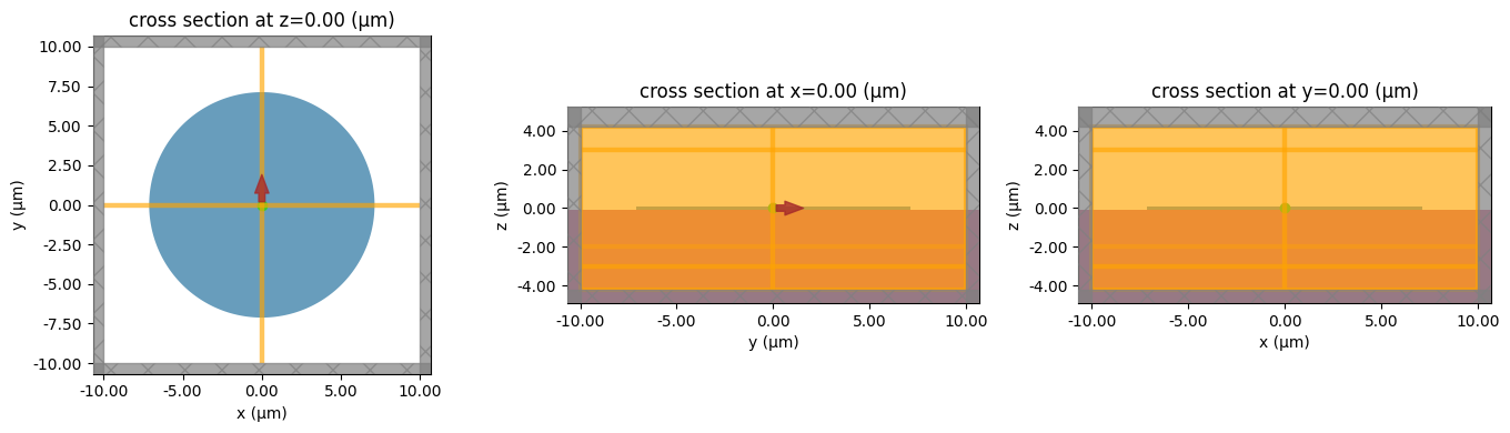
# Plot and visualize the geometry
fig, ax = plt.subplots(1, 3, tight_layout=True, figsize=(14, 4))
sim_with_cbg.plot(z=0, ax=ax[0])
sim_with_cbg.plot(x=0, freq=freq0, ax=ax[1])
sim_with_cbg.plot(y=0, freq=freq0, ax=ax[2])
plt.show()

fig, ax = plt.subplots(1, 3, tight_layout=True, figsize=(14, 4))
sim_without_cbg.plot(z=0, ax=ax[0])
sim_without_cbg.plot(x=0, freq=freq0, ax=ax[1])
sim_without_cbg.plot(y=0, freq=freq0, ax=ax[2])
plt.show()
# Run the simulation
sim_with_cbg_data = web.run(sim_with_cbg, task_name="hBN_with_cbg_2")
sim_without_cbg_data = web.run(sim_without_cbg, task_name="hBN_without_cbg_2")
12:10:10 EDT Created task 'hBN_with_cbg_2' with task_id
             'fdve-a964f30b-bc7d-4ad7-8a9e-e0b6fce6ae3f' and task_type 'FDTD'.
             View task using web UI at
             'https://tidy3d.simulation.cloud/workbench?taskId=fdve-a964f30b-bc7
             d-4ad7-8a9e-e0b6fce6ae3f'.
Task folder: 'default'.
Output()
12:10:15 EDT Maximum FlexCredit cost: 0.115. Minimum cost depends on task
             execution details. Use 'web.real_cost(task_id)' to get the billed
             FlexCredit cost after a simulation run.
12:10:16 EDT status = queued
             To cancel the simulation, use 'web.abort(task_id)' or
             'web.delete(task_id)' or abort/delete the task in the web UI.
             Terminating the Python script will not stop the job running on the
             cloud.
Output()
12:10:24 EDT status = preprocess
12:10:29 EDT starting up solver
running solver
Output()
Output()
12:11:50 EDT status = postprocess
12:15:49 EDT status = success
12:15:51 EDT View simulation result at
             'https://tidy3d.simulation.cloud/workbench?taskId=fdve-a964f30b-bc7
             d-4ad7-8a9e-e0b6fce6ae3f'.
Output()
12:21:59 EDT loading simulation from simulation_data.hdf5
12:22:06 EDT WARNING: Simulation final field decay value of 0.113 is greater
             than the simulation shutoff threshold of 1e-05. Consider running
             the simulation again with a larger 'run_time' duration for more
             accurate results.
12:22:07 EDT Created task 'hBN_without_cbg_2' with task_id
             'fdve-421c1a26-4e5b-475a-940a-47f13d2c4f57' and task_type 'FDTD'.
             View task using web UI at
             'https://tidy3d.simulation.cloud/workbench?taskId=fdve-421c1a26-4e5
             b-475a-940a-47f13d2c4f57'.
Task folder: 'default'.
Output()
12:22:08 EDT Maximum FlexCredit cost: 0.057. Minimum cost depends on task
             execution details. Use 'web.real_cost(task_id)' to get the billed
             FlexCredit cost after a simulation run.
12:22:09 EDT status = queued
             To cancel the simulation, use 'web.abort(task_id)' or
             'web.delete(task_id)' or abort/delete the task in the web UI.
             Terminating the Python script will not stop the job running on the
             cloud.
Output()
12:22:27 EDT starting up solver
running solver
Output()
Output()
12:23:15 EDT status = postprocess
12:29:49 EDT status = success
12:29:51 EDT View simulation result at
             'https://tidy3d.simulation.cloud/workbench?taskId=fdve-421c1a26-4e5
             b-475a-940a-47f13d2c4f57'.
Output()
12:33:20 EDT loading simulation from simulation_data.hdf5
12:33:23 EDT WARNING: Simulation final field decay value of 0.0634 is greater
             than the simulation shutoff threshold of 1e-05. Consider running
             the simulation again with a larger 'run_time' duration for more
             accurate results.
Looking at the Energy Coupled Into the Optical Fiber
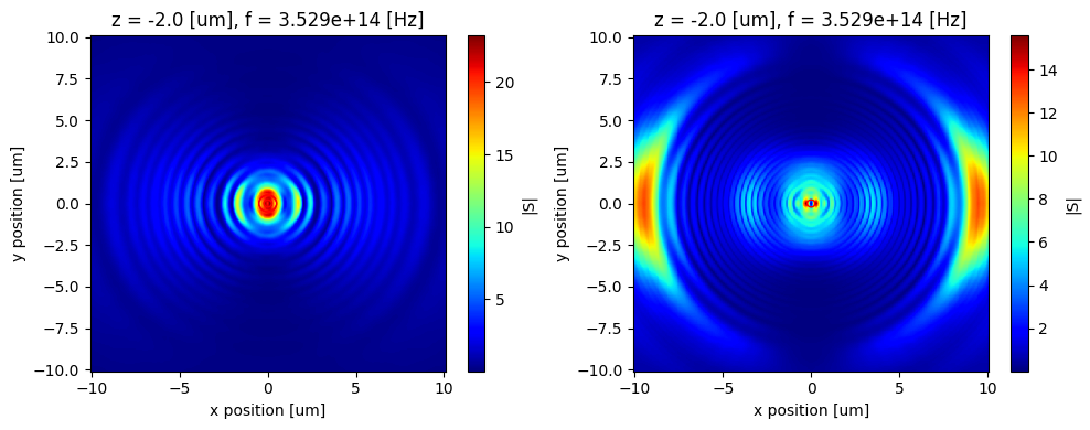
We will now plot the calculated magnitude of the Poynting vector at the various z positions.
We are primarily interested in the Poynting vector that couples the dipole emission to the fiber propagation.
It makes sense to look at 2 things: the z component and the magnitude of the Poynting vector. The z component is the energy flow into the fiber which is our signal of interest.
sim_monitor_names = ["fieldmonitor_8", "fieldmonitor_7", "fieldmonitor_6"]
zvals = [-1, -3, 3]
fields = ["S", "Sz"]

NA_1 = 0.22
NA_2 = 0.5
n_glass = 1.5

for field in fields:
    for i in range(len(sim_monitor_names)):
        s = sim_with_cbg_data._get_scalar_field(
            field_monitor_name=sim_monitor_names[i], field_name=field, val="abs"
        )
        plot_data = s.sel(z=zvals[i], method="nearest").sel(f=freq0, method="nearest")

        s = sim_without_cbg_data._get_scalar_field(
            field_monitor_name=sim_monitor_names[i], field_name=field, val="abs"
        )
        plot_data_2 = s.sel(z=zvals[i], method="nearest").sel(f=freq0, method="nearest")

        fig, ax = plt.subplots(1, 2, tight_layout=True, figsize=(10, 4))
        plot_data.plot(x="x", y="y", ax=ax[0], cmap="jet", label="With CBG")

        plot_data_2.plot(x="x", y="y", ax=ax[1], cmap="jet", label="Without CBG")

        ax[0].add_patch(
            mpatches.Circle(
                center=(0, 0),
                radius=NA_1 * abs(zvals[i]),
                edgecolor="red",
                linestyle="-",
                linewidth=1,
                fill=False,
                label="NA = 0.22",
                xy=(0, 0),
            )
        )
        ax[0].add_patch(
            mpatches.Circle(
                center=(0, 0),
                radius=NA_2 * abs(zvals[i]),
                edgecolor="red",
                linestyle="-",
                linewidth=1,
                fill=False,
                label="NA = 0.5",
                xy=(0, 0),
            )
        )

        ax[1].add_patch(
            mpatches.Circle(
                center=(0, 0),
                radius=NA_1 * abs(zvals[i]),
                edgecolor="red",
                linestyle="-",
                linewidth=1,
                fill=False,
                label="NA = 0.22",
                xy=(0, 0),
            )
        )
        ax[1].add_patch(
            mpatches.Circle(
                center=(0, 0),
                radius=NA_2 * abs(zvals[i]),
                edgecolor="red",
                linestyle="-",
                linewidth=1,
                fill=False,
                label="NA = 0.5",
                xy=(0, 0),
            )
        )
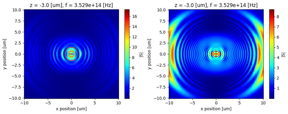
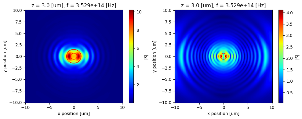
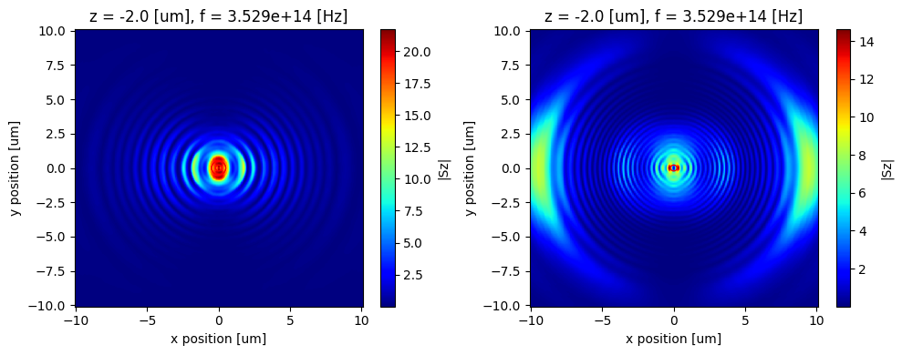
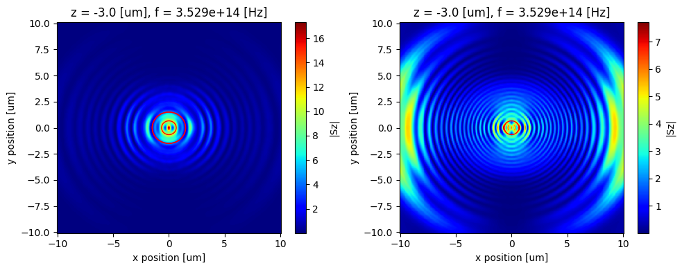

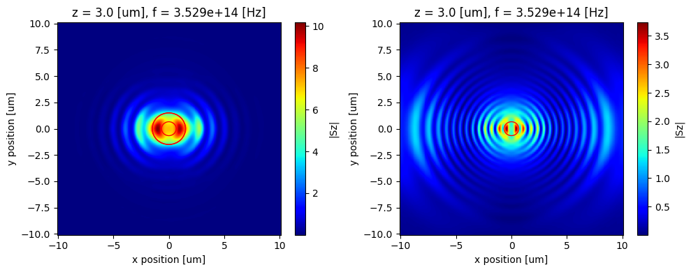
The smaller and larger red circle corresponds to $z*NA$ values of 0.22 and 0.5 respectively.
The message here is that a higher NA fiber will be able to collect a lot more emission from the dipole compared to lower NA.
This optimization can be improved further by doing a inverse design computation for extracting maximal amount of emission into the fiber. The objective function should be the flux contained inside the circle defined by the fiber NA.
As an example this paper Inverse-designed photon extractors for optically addressable defect qubits couples maximum emission into free space.
An extension of this to a medium of glass should be straightforward. Due to scale invariance, likely everything should just be scaled down by the refractive index assuming n is constant for a small wavelength range.
Now we look a simple comparison between the grating and non grating case, comparing the amount of power coupled into fiber $$\int \vec S . d\vec A = S_z * \pi r^2$$ within the small radius for the two assumed NA values.
This should give an idea of the advantage that the grating gives.
# Create mask for circle of radius NA_1 * |z|
NA = 0.22
zval = -3
radius = NA * abs(zval)

# Pull out the data with CBG
sz_data = sim_with_cbg_data._get_scalar_field(
    field_monitor_name="fieldmonitor_7", field_name="Sz", val="abs"
)
sz_slice = sz_data.sel(z=-3, method="nearest").sel(f=freq0, method="nearest")

X, Y = np.meshgrid(sz_slice.x, sz_slice.y, indexing="ij")
mask = (X**2 + Y**2) <= radius**2

# Area element
dx = np.abs(sz_slice.x[1] - sz_slice.x[0])
dy = np.abs(sz_slice.y[1] - sz_slice.y[0])
area_element = dx * dy

# Integrate CBG data with the mask
power_in_circle = np.sum(sz_slice.values[mask]) * area_element
print(f"With grating, power within radius {radius:.2f}: {power_in_circle:.4e}")

# Pull out the data without CBG
sz_data = sim_without_cbg_data._get_scalar_field(
    field_monitor_name="fieldmonitor_7", field_name="Sz", val="abs"
)
sz_slice = sz_data.sel(z=-3, method="nearest").sel(f=freq0, method="nearest")

X, Y = np.meshgrid(sz_slice.x, sz_slice.y, indexing="ij")
mask = (X**2 + Y**2) <= radius**2

# Area element
dx = np.abs(sz_slice.x[1] - sz_slice.x[0])
dy = np.abs(sz_slice.y[1] - sz_slice.y[0])
area_element = dx * dy

# Integrate with the mask
power_in_circle = np.sum(sz_slice.values[mask]) * area_element
print(f"Without grating, power within radius {radius:.2f}: {power_in_circle:.4e}")
With grating, power within radius 0.66: 4.3331e+01
Without grating, power within radius 0.66: 1.1036e+01
This tells us that the grating is 3x more efficient in coupling dipole emitter radiation into a fiber.