Author: Abhishek Das, North Carolina State University
In this notebook, we construct a novel design of a Gallium Arsenide (GaAs) cavity and evaluate its quality Q factor and far-field emission. We also calculate the percentage coupled into a regular Gaussian mode.
import gdstk
import matplotlib.pyplot as plt
import numpy as np
import tidy3d as td
import tidy3d.web as web
from tidy3d.plugins.resonance import ResonanceFinder
Simulation Setup
Define optical range, materials, and other global variables needed for the cavity.
lambda_min = 0.8
lambda_max = 1.1

monitor_lambda = np.linspace(lambda_min, lambda_max, 401)
monitor_freq = td.constants.C_0 / monitor_lambda

automesh_per_wvl = 40

sim_size = Lx, Ly, Lz = (5.5, 5.5, 2)
offset_monitor = 0.4  # monitor position in the vertical direction

vacuum = td.Medium(permittivity=1, name="vacuum")
GaAs_permittivity = 3.55**2
GaAs = td.Medium(permittivity=GaAs_permittivity, name="GaAs")

freq0 = 302.675e12
fwidth = 144.131e12
freq0 = 302.675e12

t_start = 10 / fwidth  # from inspection
t_stop = 22e-12

slab_side_length = 10
slab_height = 0.2
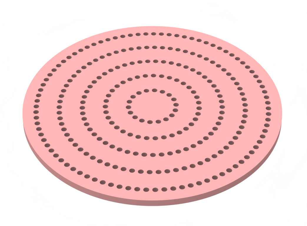
Then, define the bullseye nanocavity structure starting with a GaAs slab.
slab = td.Structure(
    geometry=td.Box(
        center=(0, 0, 0), size=(slab_side_length, slab_side_length, slab_height)
    ),
    medium=GaAs,
)
Add the aperiodic concentric rings and define the material as air to create the etched regions. Here, we use gdstk to build the rings as ellipsis objects with predefined inner and outer radii.
lib = gdstk.Library()
cell = lib.new_cell("BULLSEYE")
central_inner_radius = 0.355 + 0.027190402264497166
ring_width = 0.07 + np.array(
[
-0.04835278,
-0.01293301,
0.03173962,
0.02891523,
0.02110662,
0.02439804,
0.02123075,
]
) # rings' width
ring_height = 0.2
theta1 = 3 * np.pi / 180
theta2 = 87 * np.pi / 180
ringsNumbers = 7
vertexIncrement = 0.1075
ringNumber = 7
xOrigin = 0
yOrigin = 0
inner_radius = central_inner_radius
for i in range(ringsNumbers):
outer_radius = inner_radius + ring_width[i]
for j in range(4):
gcSlice = gdstk.ellipse(
(xOrigin, yOrigin),
inner_radius,
outer_radius,
theta1 + j * np.pi / 2,
theta2 + j * np.pi / 2,
layer=1,
datatype=1,
tolerance=0.0001,
)
cell.add(gcSlice)
inner_radius = outer_radius + vertexIncrement
gc_etch = td.Geometry.from_gds(
cell, gds_layer=1, axis=2, slab_bounds=(-ring_height / 2, ring_height / 2)
)
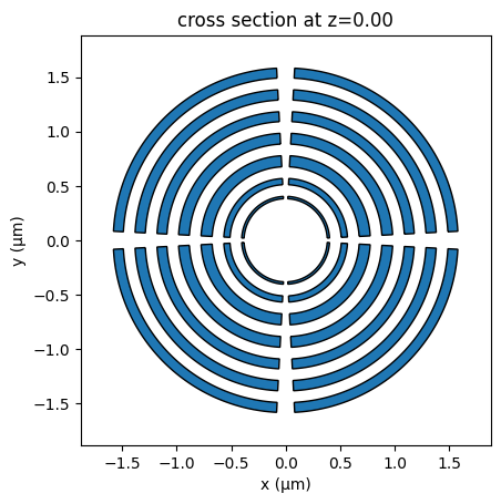
fig = plt.figure()
ax = gc_etch.plot(z=0, ax=fig.add_subplot(111))
ax.set_xlabel("x (µm)")
ax.set_ylabel("y (µm)")
plt.show()
mat_etch = td.Medium(permittivity=1, name="air")
etch = td.Structure(geometry=gc_etch, medium=mat_etch, name="etch")
An Ex-oriented dipole source is placed at the center of the cavity.
dipole_source = td.PointDipole(
    center=(0, 0, 0),
    source_time=td.GaussianPulse(freq0=freq0, fwidth=fwidth),
    polarization="Ex",
    name="dipole_source",
)
Define 4 different time domain monitors in different spatial locations. Recording in the time domain is used as this is what is needed to calculate resonance data, as will be shown later.
time_monitor_1 = td.FieldTimeMonitor(
    name="time_monitor_1", size=[0, 0, 0], center=[0.1, 0.1, 0], start=t_start
)

time_monitor_2 = td.FieldTimeMonitor(
    name="time_monitor_2", size=[0, 0, 0], center=[0.1, 0.2, 0], start=t_start
)

time_monitor_3 = td.FieldTimeMonitor(
    name="time_monitor_3", size=[0, 0, 0], center=[0.2, 0.2, 0], start=t_start
)

time_monitor_4 = td.FieldTimeMonitor(
    name="time_monitor_4", size=[0, 0, 0], center=[0.2, 0.1, 0], start=t_start
)

time_monitors = [time_monitor_1, time_monitor_2, time_monitor_3, time_monitor_4]
Define far field projection monitor. Here we would like to obtain the projected far field in polar coordinates.
far_field_monitor = td.FieldProjectionAngleMonitor(
    center=(0, 0, offset_monitor),
    size=(td.inf, td.inf, 0),
    name="far_field_monitor",
    freqs=monitor_freq,
    normal_dir="-",
    phi=np.linspace(0, 2 * np.pi, 361),
    theta=np.linspace(0, np.pi, 181),
)
Combine all objects into simulation object.
sim = td.Simulation(
    center=(0, 0, 0),
    size=sim_size,
    grid_spec=td.GridSpec.auto(
        wavelength=(lambda_min + lambda_max) / 2, min_steps_per_wvl=automesh_per_wvl
    ),
    run_time=t_stop,
    sources=[dipole_source],
    monitors=time_monitors + [far_field_monitor],
    structures=[slab, etch],
    medium=vacuum,
    shutoff=1e-7,
    symmetry=[-1, 1, 0],
)
19:15:28 Eastern Daylight Time WARNING: Field projection monitor
                               'far_field_monitor' has observation points set up
                               such that the monitor is projecting backwards
                               with respect to its 'normal_dir'. If this was not
                               intentional, please take a look at the
                               documentation associated with this type of
                               projection monitor to check how the observation
                               point coordinate system is defined.
Submit the Simulation and Visualize the Result
Now, we submitt the simulation to the cloud using the web API. After running the simulation, print out the simulation log for inspection.
sim_data = web.run(simulation=sim, task_name="Aperiodic ring cavity")
print(sim_data.log)
                               WARNING: Simulation has 1.73e+06 time steps. The
                               'run_time' may be unnecessarily large, unless
                               there are very long-lived resonances.
19:15:29 Eastern Daylight Time Created task 'Aperiodic ring cavity' with task_id
                               'fdve-a00b1637-0dfc-41ea-949e-45587ff34a62' and
                               task_type 'FDTD'.
                               View task using web UI at
                               'https://tidy3d.simulation.cloud/workbench?taskId
                               =fdve-a00b1637-0dfc-41ea-949e-45587ff34a62'.
Task folder: 'default'.
Output()
19:15:31 Eastern Daylight Time Maximum FlexCredit cost: 22.540. Minimum cost
                               depends on task execution details. Use
                               'web.real_cost(task_id)' to get the billed
                               FlexCredit cost after a simulation run.
status = success
Output()
19:15:58 Eastern Daylight Time loading simulation from simulation_data.hdf5
19:15:59 Eastern Daylight Time WARNING: Field projection monitor
                               'far_field_monitor' has observation points set up
                               such that the monitor is projecting backwards
                               with respect to its 'normal_dir'. If this was not
                               intentional, please take a look at the
                               documentation associated with this type of
                               projection monitor to check how the observation
                               point coordinate system is defined.
                               WARNING: Simulation final field decay value of
                               1.46e-05 is greater than the simulation shutoff
                               threshold of 1e-07. Consider running the
                               simulation again with a larger 'run_time'
                               duration for more accurate results.
                               WARNING: Warning messages were found in the
                               solver log. For more information, check
                               'SimulationData.log' or use
                               'web.download_log(task_id)'.
[14:23:47] WARNING: Field projection monitor 'far_field_monitor' has observation
           points set up such that the monitor is projecting backwards with
           respect to its 'normal_dir'. If this was not intentional, please take
           a look at the documentation associated with this type of projection
           monitor to check how the observation point coordinate system is
           defined.
           USER: Simulation domain Nx, Ny, Nz: [848, 848, 134]
           USER: Applied symmetries: (-1, 1, 0)
           USER: Number of computational grid points: 2.4681e+07.
           USER: Subpixel averaging method: SubpixelSpec(attrs={},
           dielectric=PolarizedAveraging(attrs={}, type='PolarizedAveraging'),
           metal=Staircasing(attrs={}, type='Staircasing'),
           pec=PECConformal(attrs={}, type='PECConformal',
           timestep_reduction=0.3), lossy_metal=SurfaceImpedance(attrs={},
           type='SurfaceImpedance', timestep_reduction=0.0),
           type='SubpixelSpec')
           USER: Number of time steps: 1.7300e+06
           USER: Automatic shutoff factor: 1.00e-07
           USER: Time step (s): 1.2717e-17
           USER:

           USER: Compute source modes time (s):     0.1118
[14:23:48] USER: Rest of setup time (s):            0.8236
[14:24:05] USER: Compute monitor modes time (s):    0.0001
[15:27:40] USER: Solver time (s):                   3829.1860
           USER: Time-stepping speed (cells/s):     1.20e+10
[15:27:49] USER: Post-processing time (s):          8.3246

 ====== SOLVER LOG ======

Processing grid and structures...
Building FDTD update coefficients...
Solver setup time (s):             14.9848

Running solver for 1730033 time steps...
- Time step    434 / time 5.52e-15s (  0 % done), field decay: 1.00e+00
- Time step  69201 / time 8.80e-13s (  4 % done), field decay: 6.75e-04
- Time step 138402 / time 1.76e-12s (  8 % done), field decay: 1.96e-04
- Time step 207603 / time 2.64e-12s ( 12 % done), field decay: 2.65e-04
- Time step 276805 / time 3.52e-12s ( 16 % done), field decay: 6.20e-04
- Time step 346006 / time 4.40e-12s ( 20 % done), field decay: 9.19e-04
- Time step 415207 / time 5.28e-12s ( 24 % done), field decay: 1.04e-03
- Time step 484409 / time 6.16e-12s ( 28 % done), field decay: 9.58e-04
- Time step 553610 / time 7.04e-12s ( 32 % done), field decay: 7.26e-04
- Time step 622811 / time 7.92e-12s ( 36 % done), field decay: 4.52e-04
- Time step 692013 / time 8.80e-12s ( 40 % done), field decay: 2.02e-04
- Time step 761214 / time 9.68e-12s ( 44 % done), field decay: 5.63e-05
- Time step 830415 / time 1.06e-11s ( 48 % done), field decay: 2.93e-06
- Time step 899617 / time 1.14e-11s ( 52 % done), field decay: 2.18e-05
- Time step 968818 / time 1.23e-11s ( 56 % done), field decay: 7.14e-05
- Time step 1038019 / time 1.32e-11s ( 60 % done), field decay: 1.18e-04
- Time step 1107221 / time 1.41e-11s ( 64 % done), field decay: 1.45e-04
- Time step 1176422 / time 1.50e-11s ( 68 % done), field decay: 1.38e-04
- Time step 1245623 / time 1.58e-11s ( 72 % done), field decay: 1.09e-04
- Time step 1314825 / time 1.67e-11s ( 76 % done), field decay: 6.96e-05
- Time step 1384026 / time 1.76e-11s ( 80 % done), field decay: 3.51e-05
- Time step 1453227 / time 1.85e-11s ( 84 % done), field decay: 1.17e-05
- Time step 1522429 / time 1.94e-11s ( 88 % done), field decay: 9.06e-07
- Time step 1591630 / time 2.02e-11s ( 92 % done), field decay: 1.65e-06
- Time step 1660831 / time 2.11e-11s ( 96 % done), field decay: 7.83e-06
- Time step 1730032 / time 2.20e-11s (100 % done), field decay: 1.46e-05
Time-stepping time (s):            3543.4963
Field projection time (s):         265.7101
Data write time (s):               4.9940
Use the Tidy3D Resonance Finder to calculate Q factor and other resonance data:
resonance_finder = ResonanceFinder(freq_window=(monitor_freq[-1], monitor_freq[0]))
resonance_data = resonance_finder.run(signals=sim_data.data)
resonance_data.to_dataframe()
| decay | Q | amplitude | phase | error | |
|---|---|---|---|---|---|
| freq | |||||
| 2.643023e+14 | 2.361523e+12 | 351.607965 | 77.807785 | 1.377193 | 0.008803 |
| 2.794917e+14 | 2.320479e+12 | 378.391288 | 67.513793 | -1.689715 | 0.009099 |
| 3.142660e+14 | 1.413021e+12 | 698.712741 | 179.443262 | -3.089416 | 0.003164 |
| 3.193734e+14 | 1.102090e+11 | 9103.986954 | 167.987280 | -2.094138 | 0.000362 |
| 3.268678e+14 | 3.906235e+11 | 2628.836765 | 209.390600 | -1.892530 | 0.000806 |
| 4.013446e+14 | 4.829837e+12 | 261.056679 | 586.826250 | 2.013540 | 0.017215 |
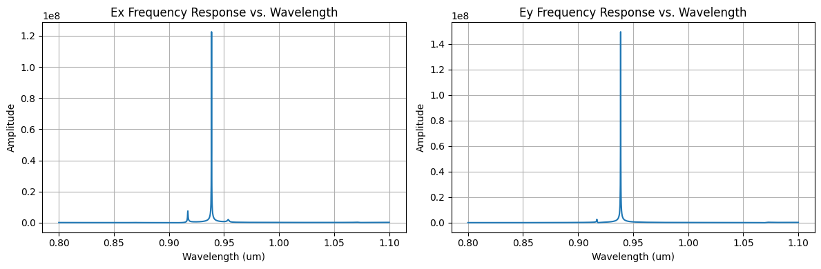
We use FFT to calculate the frequency response from the time domain data.
fig, ax = plt.subplots(1, 2, tight_layout=True, figsize=(12, 4))

time_monitor_names = [monitor.name for monitor in time_monitors]

time_response_Ex = np.zeros_like(sim_data["time_monitor_1"].Ex.squeeze())
time_response_Ey = np.zeros_like(sim_data["time_monitor_1"].Ey.squeeze())

for monitor_name in time_monitor_names:
    time_response_Ex += sim_data[monitor_name].Ex.squeeze()
    time_response_Ey += sim_data[monitor_name].Ey.squeeze()

time_response_Ex /= len(time_monitor_names)
time_response_Ey /= len(time_monitor_names)

# Perform FFT and get the frequency response
freq_response_Ex = np.abs(np.fft.fft(time_response_Ex))
freq_response_Ey = np.abs(np.fft.fft(time_response_Ey))

# Calculate the frequency values
freqs_Ex = np.linspace(0, 1 / sim_data.simulation.dt, len(time_response_Ex))
freqs_Ey = np.linspace(0, 1 / sim_data.simulation.dt, len(time_response_Ey))

# Calculate the corresponding wavelengths
with np.errstate(divide="ignore"):
    wavelengths_Ex = td.constants.C_0 / freqs_Ex
    wavelengths_Ey = td.constants.C_0 / freqs_Ey

# Select the indices within the monitor frequency range
plot_inds_Ex = np.where((monitor_freq[-1] < freqs_Ex) & (freqs_Ex < monitor_freq[0]))
plot_inds_Ey = np.where((monitor_freq[-1] < freqs_Ey) & (freqs_Ey < monitor_freq[0]))

# Plot the frequency response with respect to wavelength
ax[0].plot(wavelengths_Ex[plot_inds_Ex], freq_response_Ex[plot_inds_Ex])
ax[0].set_xlabel("Wavelength (um)")
ax[0].set_ylabel("Amplitude")
ax[0].set_title("Ex Frequency Response vs. Wavelength")
ax[0].grid(True)

ax[1].plot(wavelengths_Ey[plot_inds_Ey], freq_response_Ey[plot_inds_Ey])
ax[1].set_xlabel("Wavelength (um)")
ax[1].set_ylabel("Amplitude")
ax[1].set_title("Ey Frequency Response vs. Wavelength")
ax[1].grid(True)

plt.show()
Get far field data for plotting and overlap calculations.
f_index = 185
far_field_data = sim_data[far_field_monitor.name]
Etheta = far_field_data.Etheta.isel(f=f_index, r=0).values
Ephi = far_field_data.Ephi.isel(f=f_index, r=0).values
phi_vals = far_field_data.phi
theta_vals = far_field_data.theta
intensity = np.abs(Etheta) ** 2 + np.abs(Ephi) ** 2
intensity /= np.max(intensity)
Create a function that plots field/intensity data in polar coordinates.
from scipy.interpolate import griddata


def make_field_plot(phi, theta, vals, NA_circle=0.68):
    phi = np.array(phi)
    theta = np.array(theta)
    vals = np.array(vals)

    # Ensure periodicity in phi
    phi_extended = np.concatenate((phi, [phi[0] + 2 * np.pi]))
    vals_extended = np.hstack((vals, vals[:, [0]]))

    # Dense grid for smooth interpolation
    phi_dense, theta_dense = np.meshgrid(
        np.linspace(phi_extended.min(), phi_extended.max(), 360),
        np.linspace(theta.min(), theta.max(), 180),
    )

    # Interpolate data onto dense grid
    points = np.array([(p, t) for t in theta for p in phi_extended])
    values = vals_extended.flatten()

    grid_vals = griddata(
        points, values, (phi_dense, theta_dense), method="cubic", fill_value=0
    )

    fig, ax = plt.subplots(subplot_kw={"projection": "polar"}, figsize=(6, 5))
    c = ax.pcolormesh(
        phi_dense, theta_dense * 180 / np.pi, grid_vals, cmap="jet", shading="auto"
    )
    fig.colorbar(c, ax=ax, orientation="vertical", label="Normalized Intensity (a.u.)")

    ax.set_ylim(0, 90)
    ax.set_title("Far Field Intensity Polar Plot", fontsize=14)
    ax.set_xlabel("$\\phi$ (rad)")
    ax.set_ylabel("$\\theta$ (deg)", labelpad=20)
    ax.yaxis.set_label_coords(
        -0.1, 0.5
    )  # Move the label leftward (x < 0.0) and vertically centered (y = 0.5)

    # Add white circle corresponding to NA
    theta_NA_deg = np.degrees(np.arcsin(NA_circle))
    phi_circle = np.linspace(0, 2 * np.pi, 500)
    theta_circle = np.full_like(phi_circle, theta_NA_deg)

    ax.plot(phi_circle, theta_circle, color="white", linestyle="--", linewidth=2)

    # Annotate NA circle near phi = 45 degrees
    phi_annot = np.pi / 4  # 45 degrees
    theta_annot = theta_NA_deg + 2  # a bit outward for visibility

    ax.text(
        phi_annot,
        theta_annot,
        f"NA = {NA_circle}",
        color="white",
        ha="center",
        va="bottom",
        fontsize=10,
        weight="bold",
    )

    plt.tight_layout()
    plt.show()
make_field_plot(phi_vals, theta_vals, intensity)
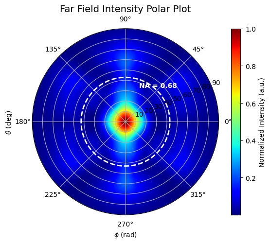
Using the $E$ data from this simulation, we now can calculate the power overlap with that of a Gaussian beam:
# Parameters
NA = 0.68
n = 1.0
theta_max = np.arcsin(NA / n)  # max angle for the Gaussian beam
theta_0 = theta_max  # beam divergence angle

# Grids: theta_vals, phi_vals, intensity are assumed already defined
phi_grid, theta_grid = np.meshgrid(phi_vals, theta_vals)

# Differential elements (assume uniform)
dtheta = np.diff(theta_vals)[0]
dphi = np.diff(phi_vals)[0]
dOmega = np.sin(theta_grid) * dtheta * dphi  # solid angle element

# Define normalized Gaussian beam intensity profile
E_gauss = np.exp(-((theta_grid / theta_0) ** 2))  # (amplitude)
I_gauss = E_gauss**2  # intensity (|E|^2)

# --- Normalize E_sim (optional if already normalized) ---
I_sim = intensity  # if intensity = |E|^2
E_sim = np.sqrt(I_sim)

# --- Numerator: |<E_sim | E_gauss>|^2 ---
overlap = np.sum(E_sim * E_gauss * dOmega)
numerator = np.abs(overlap) ** 2

# --- Denominator: energy normalization ---
norm_sim = np.sum(I_sim * dOmega)
norm_gauss = np.sum(I_gauss * dOmega)

# --- Efficiency ---
eta = numerator / (norm_sim * norm_gauss)
percentage_overlap = eta * 100

print(
    f"Percentage of power coupled into Gaussian beam (NA={NA}): {percentage_overlap:.2f}%"
)
Percentage of power coupled into Gaussian beam (NA=0.68): 69.21%