Author: Jungmin Kim, University of Wisconsin-Madison

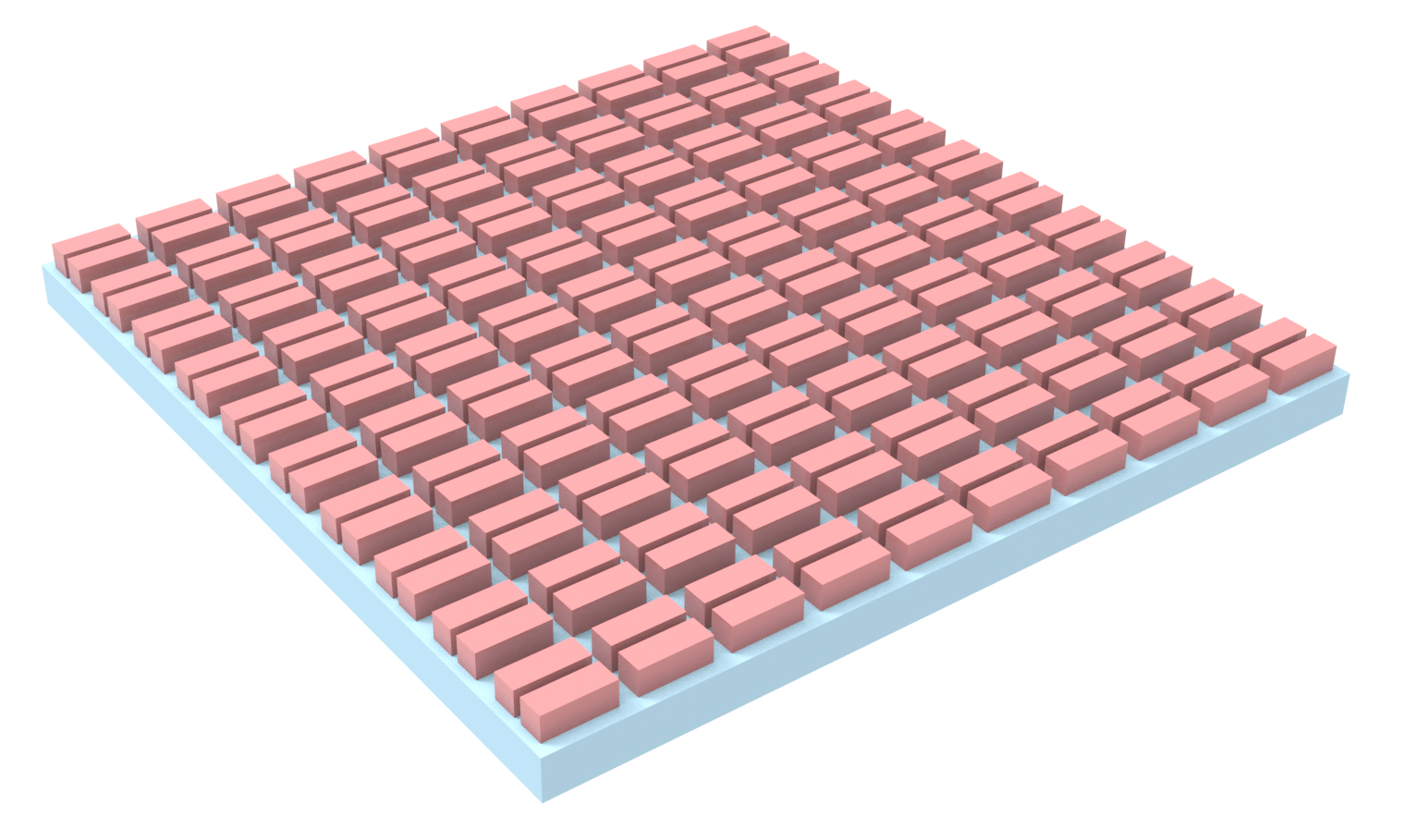
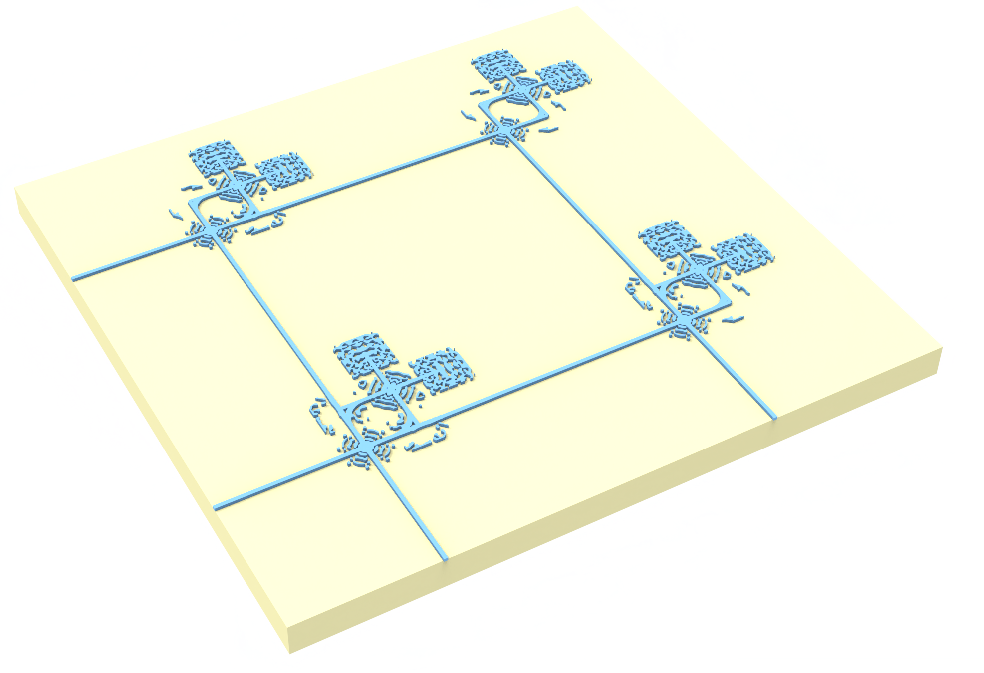
In this notebook, we demonstrate matrix-matrix multiplication using 2-by-2 photonic systolic array, an array of optical processing elements (PEs) that receives columns of matrices $A, B \in \mathbb{R}^{K\times 2}$ encoded as synchronized pulse trains. The array performs inner product between column vectors through homodyne detection across the device, effectively computing $A^T B \in \mathbb{R}^{2\times 2}$ in a parallel manner.

Specifically, pulse trains of length $K$ are injected along vertical ($A$) and horizontal ($B$) waveguides. At each PE at position $(m,n)$ where the pulse trains for column $A_m$ and $B_n$ encounter, a fraction of the optical energy of each pulse is routed to a pair of detectors, while the remaining portion continues to propagate to the next PEs. This enables cascaded accumulation of the signal across the array.

The full project dataset and Python implementation are available at GitHub. Running this notebook requires ~60 FlexCredits and ~10 minutes of simulation time.

[1]:

import pickle

import matplotlib
import matplotlib.pyplot as plt
import numpy as np

matplotlib.rcParams.update({"font.size": 7})
matplotlib.rcParams["font.family"] = "Arial"

import tidy3d as td
import tidy3d.web as web
from tidy3d.plugins.adjoint.utils.filter import BinaryProjector, ConicFilter
from tidy3d.plugins.mode import ModeSolver

td.config.logging_level = "ERROR"

Define Simulation¶

Each processing element consists of the following components:

Crossing that allows two waveguide signals to propagate orthogonally with minimal crosstalk,
Beam splitter that divides the input optical power equally (50:50), while introducing a 90-degree phase difference between two output arms,
Branches that further split the optical power according to predefined ratios (1:1, 1:2, 1:3), with controlled phase.
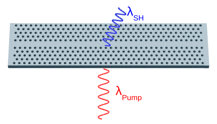
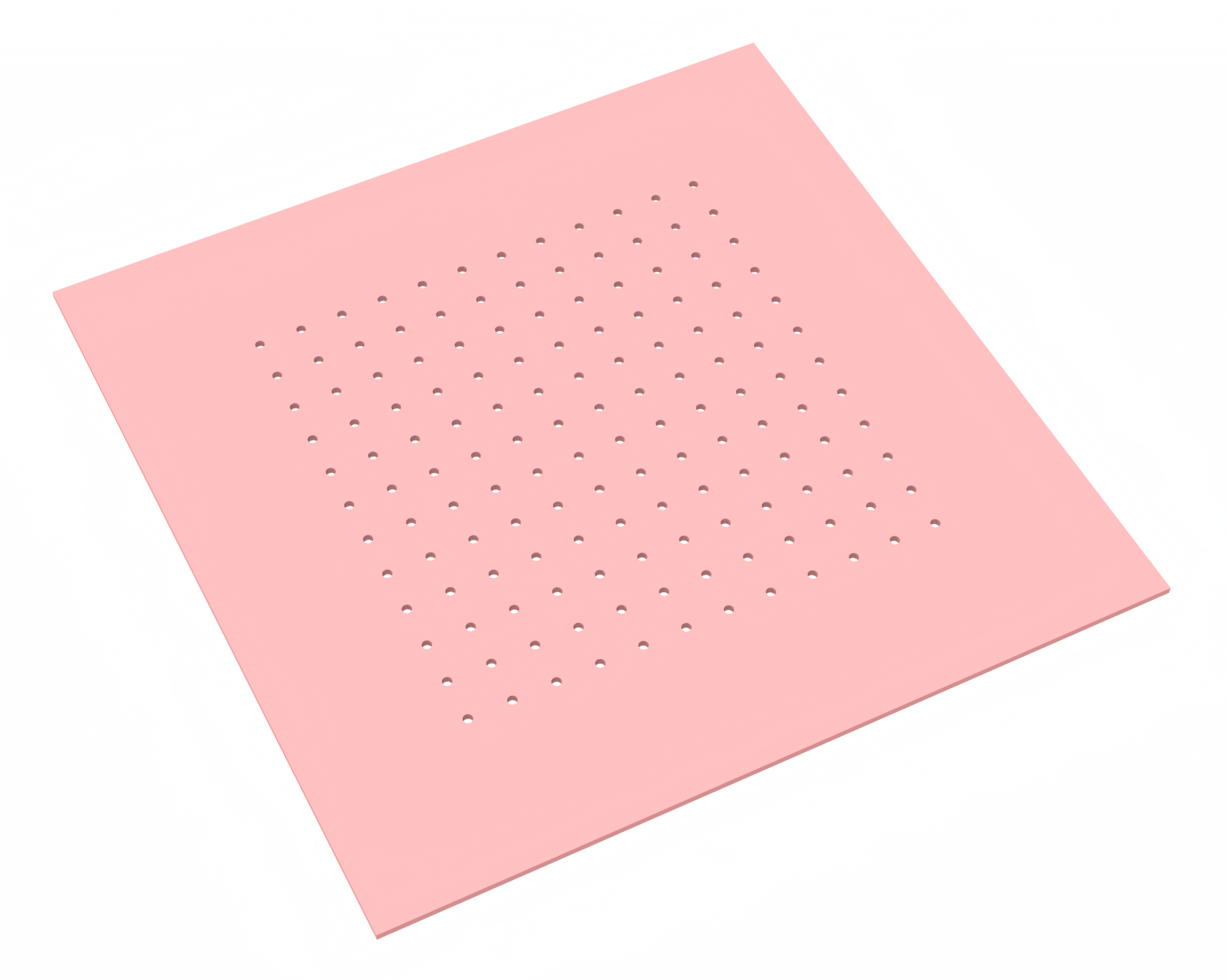
Grating couplers that direct in-plane waveguide signal to out-of-plane radiation.

All submodules are pre-optimized using adjoint method.

[2]:

## Spectral parameters
wavelength = 1.55
k0 = 2 * np.pi / wavelength
freq0 = td.C_0 / wavelength
freq_list = freq0 * np.linspace(0.95, 1.05, 101)

# beta_start = 10.0
l_des = 3.5
pixel_size = l_des / 350

radius = 120e-3  # minimum fab size
smoothen = ConicFilter(radius=radius, design_region_dl=pixel_size)
Si = td.material_library["cSi"]["Palik_Lossless"]
SiO2 = td.material_library["SiO2"]["Palik_Lossless"]

module_names = ["cross", "BS", "1", "2", "3", "4"]

## Load epsilon parameters for all submodules.
eps_opt = np.load("misc/eps_opt.npz")

fig, ax = plt.subplots(
    2, 4, figsize=(6, 3), sharex=True, sharey=True, tight_layout=True
)
ax = ax.T.reshape(-1)
[ax[i].matshow(np.real(eps)) for i, eps in enumerate(eps_opt.values())]
[ax[i].set_title(keys) for i, keys in enumerate(eps_opt.keys())]
[ax[-1].spines[pos].set_visible(False) for pos in ["top", "bottom", "left", "right"]]
ax[-1].set(xticks=[], yticks=[])

[2]:

[[], []]

No description has been provided for this image

Now we define make_sim which generates the array of 2-by-2 processing elements and connecting waveguides, as well as mode sources and all necessary monitors.

[3]:

### Effective phase and group velocity at 1550 nm waveguide.
n_eff_phase = 1.829328179359436
n_eff_group = 4.092397301962457

### Geometry parameters
h_box = 2.0
h_clad = 0.78
h_sub = 500
w_wg = 0.3
h_wg = 0.22
dist_wg = 4.8
w_mode = dist_wg * 1.0
min_step_per_wvl = 20


def get_structure(
    eps: np.ndarray, center: tuple = (0, 0, 0), size: tuple = (l_des, l_des, h_wg)
):
    xs = np.linspace(
        center[0] - (l_des - pixel_size) / 2,
        center[0] + (l_des - pixel_size) / 2,
        eps.shape[0],
    ).tolist()
    ys = np.linspace(
        center[1] - (l_des - pixel_size) / 2,
        center[1] + (l_des - pixel_size) / 2,
        eps.shape[1],
    ).tolist()
    coords = dict(x=xs, y=ys, z=[center[2]], f=[freq0])
    eps_data = td.ScalarFieldDataArray(
        eps.reshape(eps.shape[0], eps.shape[1], 1, 1), coords=coords
    )
    field_components = {f"eps_{dim}{dim}": eps_data for dim in "xyz"}
    eps_dataset = td.PermittivityDataset(**field_components)
    custom_medium = td.CustomMedium(eps_dataset=eps_dataset)
    return td.Structure(geometry=td.Box(center=center, size=size), medium=custom_medium)


### Array parameters
N_cell = (2, 2)  # Change as (1,4) first to calculate time delay
lattice_const = wavelength / n_eff_phase * 30
dist_module = 4.0
x_cell_center = (N_cell[0] / 2 - 1 / 2 - np.arange(N_cell[0])) * lattice_const
y_cell_center = (N_cell[1] / 2 - 1 / 2 - np.arange(N_cell[1])) * lattice_const


buffer_pml_xy = 1.5 * wavelength
buffer_pml_z = 1 * wavelength
Lx = N_cell[0] * lattice_const + 2 * buffer_pml_xy
Ly = N_cell[1] * lattice_const + 2 * buffer_pml_xy
Lz = 2 * buffer_pml_z + h_clad + h_wg
z_offset = Lz / 2 - (buffer_pml_z + h_clad + h_wg / 2)

## Temporal parameters
pulse_width = 100
fwidth = freq0 / pulse_width
t_delay = 3.486268405754292e-13

run_time = (
    15 / (2 * np.pi * fwidth)
    + t_delay * (np.sum(N_cell) - 1)
    + (h_clad + h_wg) * SiO2.nk_model(freq_list)[0][50] / td.C_0
)

# structures
BOx = td.Structure(
    geometry=td.Box(
        size=(td.inf, td.inf, h_box), center=(0, 0, -(h_wg + h_box) / 2 + z_offset)
    ),
    medium=SiO2,
)
cladding = td.Structure(
    geometry=td.Box(
        size=(td.inf, td.inf, h_clad + h_wg), center=(0, 0, h_clad / 2 + z_offset)
    ),
    medium=SiO2,
)
substrate = td.Structure(
    geometry=td.Box(
        center=(0, 0, -(h_wg + h_sub) / 2 - h_box + z_offset),
        size=(td.inf, td.inf, h_sub),
    ),
    medium=Si,
)
base_structure = [BOx, cladding]
wg_x = [
    td.Structure(
        geometry=td.Box(
            center=(-dist_module + x_cell_center[i], -lattice_const / 2, z_offset),
            size=(w_wg, N_cell[1] * lattice_const, h_wg),
        ),
        medium=Si,
    )
    for i in range(N_cell[0])
]
wg_y = [
    td.Structure(
        geometry=td.Box(
            center=(-lattice_const / 2, -dist_module + y_cell_center[i], z_offset),
            size=(N_cell[0] * lattice_const, w_wg, h_wg),
        ),
        medium=Si,
    )
    for i in range(N_cell[1])
]
wg_intra_x = [
    td.Structure(
        geometry=td.Box(
            center=(x_cell_center[i], y_cell_center[j], z_offset),
            size=(w_wg, 2 * dist_module, h_wg),
        ),
        medium=Si,
    )
    for i in range(N_cell[0])
    for j in range(N_cell[1])
]
wg_intra_y = [
    td.Structure(
        geometry=td.Box(
            center=(x_cell_center[i], y_cell_center[j], z_offset),
            size=(2 * dist_module, w_wg, h_wg),
        ),
        medium=Si,
    )
    for i in range(N_cell[0])
    for j in range(N_cell[1])
]
crossings = [
    get_structure(
        eps_opt["cross"],
        center=(
            x_cell_center[i] - dist_module,
            y_cell_center[j] - dist_module,
            z_offset,
        ),
    )
    for i in range(N_cell[0])
    for j in range(N_cell[1])
]
splitter = [
    get_structure(
        eps_opt[str(j + 1)] * p + (eps_opt[str(i + 1)].T) * (1 - p),
        center=(
            x_cell_center[i] - dist_module * p,
            y_cell_center[j] - dist_module * (1 - p),
            z_offset,
        ),
    )
    for i in range(N_cell[0])
    for j in range(N_cell[1])
    for p in range(2)
]
BSs = [
    get_structure(eps_opt["BS"], center=(x_cell_center[i], y_cell_center[j], z_offset))
    for i in range(N_cell[0])
    for j in range(N_cell[1])
]
grating = [
    get_structure(
        eps_opt["grating"].T * p + eps_opt["grating"] * (1 - p),
        center=(
            x_cell_center[i] + dist_module * p,
            y_cell_center[j] + dist_module * (1 - p),
            h_wg / 4 + z_offset,
        ),
        size=(l_des, l_des, h_wg / 2),
    )
    for i in range(N_cell[0])
    for j in range(N_cell[1])
    for p in range(2)
]
grating_sub = [
    td.Structure(
        geometry=td.Box(
            center=(
                x_cell_center[i] + dist_module * p,
                y_cell_center[j] + dist_module * (1 - p),
                -h_wg / 4 + z_offset,
            ),
            size=(l_des, l_des, h_wg / 2),
        ),
        medium=Si,
    )
    for i in range(N_cell[0])
    for j in range(N_cell[1])
    for p in range(2)
]
base_structure = (
    base_structure
    + wg_x
    + wg_y
    + wg_intra_x
    + wg_intra_y
    + crossings
    + splitter
    + BSs
    + grating
    + grating_sub
)

grid_spec = td.GridSpec.auto(wavelength=wavelength, min_steps_per_wvl=min_step_per_wvl)
sim_base = td.Simulation(
    size=(Lx, Ly, Lz),
    structures=base_structure,
    grid_spec=grid_spec,
    boundary_spec=td.BoundarySpec.pml(x=True, y=True, z=True),
    run_time=run_time,
    subpixel=True,
)

## Mode sources and monitors
plane_in = td.Box(
    size=(w_mode, 0, wavelength + h_wg),
    center=(
        x_cell_center[-1] - dist_module,
        y_cell_center[-1] - lattice_const / 2,
        z_offset,
    ),
)
num_modes = 1
mode_spec = td.ModeSpec(num_modes=num_modes, target_neff=n_eff_phase)
mode_solver = ModeSolver(
    simulation=sim_base,
    plane=plane_in,
    mode_spec=mode_spec,
    freqs=[freq0],
)
mode_data = mode_solver.solve()

mnt_thru_A_flux = [
    td.FluxTimeMonitor(
        center=(x - dist_module, y - lattice_const / 2, z_offset),
        size=(w_wg, 0, h_wg),
        name="thruA_{}_{}_flux".format(nx, ny),
        interval=5,
    )
    for nx, x in enumerate(x_cell_center)
    for ny, y in enumerate(y_cell_center)
]

mnt_thru_B_flux = [
    td.FluxTimeMonitor(
        center=(x - lattice_const / 2, y - dist_module, z_offset),
        size=(0, w_wg, h_wg),
        name="thruB_{}_{}_flux".format(nx, ny),
        interval=5,
    )
    for nx, x in enumerate(x_cell_center)
    for ny, y in enumerate(y_cell_center)
]

mnt_det_C_flux = [
    td.FluxTimeMonitor(
        center=(x, y + dist_module, h_wg / 2 + h_clad * 1.1 + z_offset),
        size=(l_des, l_des, 0),
        name="detC_{}_{}_flux".format(nx, ny),
        interval=5,
    )
    for nx, x in enumerate(x_cell_center)
    for ny, y in enumerate(y_cell_center)
]

mnt_det_D_flux = [
    td.FluxTimeMonitor(
        center=(x + dist_module, y, h_wg / 2 + h_clad * 1.1 + z_offset),
        size=(l_des, l_des, 0),
        name="detD_{}_{}_flux".format(nx, ny),
        interval=5,
    )
    for nx, x in enumerate(x_cell_center)
    for ny, y in enumerate(y_cell_center)
]


mnt_det_C_field = [
    td.FieldTimeMonitor(
        center=(x + delx, y + dist_module + dely, h_wg / 2 + h_clad * 1.1 + z_offset),
        size=(0, 0, 0),
        name="detC_{}_{}_{}_{}_field".format(nx, ny, ndx, ndy),
        interval=5,
    )
    for nx, x in enumerate(x_cell_center)
    for ny, y in enumerate(y_cell_center)
    for ndx, delx in enumerate(np.arange(-l_des / 2 + l_des / 10, l_des / 2, l_des / 5))
    for ndy, dely in enumerate(np.arange(-l_des / 2 + l_des / 10, l_des / 2, l_des / 5))
]

mnt_det_D_field = [
    td.FieldTimeMonitor(
        center=(x + dist_module + delx, y + dely, h_wg / 2 + h_clad * 1.1 + z_offset),
        size=(0, 0, 0),
        name="detD_{}_{}_{}_{}_field".format(nx, ny, ndx, ndy),
        interval=5,
    )
    for nx, x in enumerate(x_cell_center)
    for ny, y in enumerate(y_cell_center)
    for ndx, delx in enumerate(np.arange(-l_des / 2 + l_des / 10, l_des / 2, l_des / 5))
    for ndy, dely in enumerate(np.arange(-l_des / 2 + l_des / 10, l_des / 2, l_des / 5))
]

freq_monitor = mode_solver.to_monitor(name="temp")
mnt_thru_A_freq = [
    freq_monitor.updated_copy(
        mode_spec=td.ModeSpec(num_modes=1, target_neff=n_eff_phase),
        size=(w_mode, 0, wavelength + h_wg),
        center=(x - dist_module, y - lattice_const / 2, z_offset),
        name="thruA_{}_{}_freq".format(nx, ny),
    )
    for nx, x in enumerate(x_cell_center)
    for ny, y in enumerate(y_cell_center)
]
mnt_thru_B_freq = [
    freq_monitor.updated_copy(
        mode_spec=mode_spec,
        size=(0, w_mode, wavelength + h_wg),
        center=(x - lattice_const / 2, y - dist_module, z_offset),
        name="thruB_{}_{}_freq".format(nx, ny),
    )
    for nx, x in enumerate(x_cell_center)
    for ny, y in enumerate(y_cell_center)
]

mnt_landscape = td.FieldMonitor(
    center=(0, 0, z_offset),
    size=(Lx, Ly, 0),
    name="field_center",
    fields=["Hz", "Ex", "Ey"],
    freqs=[freq0],
    colocate=False,
)
mnt_landscape_air = td.FieldMonitor(
    center=(0, 0, h_wg / 2 + h_clad * 1.1 + z_offset),
    size=(Lx, Ly, 0),
    name="field_air",
    freqs=[freq0],
    fields=["Ex", "Ey", "Hx", "Hy"],
    colocate=False,
)
mnt_field_freq = [mnt_landscape, mnt_landscape_air]
monitors = (
    mnt_thru_A_flux
    + mnt_thru_B_flux
    + mnt_det_C_flux
    + mnt_det_D_flux
    + mnt_det_C_field
    + mnt_det_D_field
    + mnt_thru_A_freq
    + mnt_thru_B_freq
    + mnt_field_freq
)


## Generating simulation objects as a function of input source amplitudes.
def make_sim(src_amp: tuple = (1, 0, 0, 0)):
    amp_A = src_amp[: N_cell[0]]
    amp_B = src_amp[N_cell[0] :]

    src_A = [
        td.ModeSource(
            size=(w_mode, 0, wavelength + h_wg),
            center=(
                x - dist_module,
                y_cell_center[-1] - lattice_const / 2 - 0.1 * wavelength,
                z_offset,
            ),
            source_time=td.GaussianPulse(
                freq0=freq0,
                fwidth=fwidth,
                amplitude=1e-14 + np.abs(amp_A[nx]) * np.sqrt(N_cell[1]),
                phase=0 + np.pi * (amp_A[nx] < 0),
                # offset=4 + 2*np.pi*fwidth * t_delay_prac[nx],
                offset=4 + 2 * np.pi * fwidth * t_delay * (N_cell[0] - 1 - nx),
            ),
            mode_spec=mode_spec,
            mode_index=0,
            direction="+",
            num_freqs=9,
            name=f"A_{nx}",
        )
        for nx, x in enumerate(x_cell_center)
    ]

    src_B = [
        td.ModeSource(
            size=(0, w_mode, wavelength + h_wg),
            center=(
                x_cell_center[-1] - lattice_const / 2 - 0.1 * wavelength,
                y - dist_module,
                z_offset,
            ),
            source_time=td.GaussianPulse(
                freq0=freq0,
                fwidth=fwidth,
                amplitude=1e-14 + np.abs(amp_B[ny]) * np.sqrt(N_cell[0]),
                phase=-np.pi / 2 + np.pi * (amp_B[ny] < 0),
                # offset=4 + 2*np.pi*fwidth * t_delay_prac[ny],
                offset=4 + 2 * np.pi * fwidth * t_delay * (N_cell[1] - 1 - ny),
            ),
            mode_spec=mode_spec,
            mode_index=0,
            direction="+",
            num_freqs=9,
            name=f"B_{ny}",
        )
        for ny, y in enumerate(y_cell_center)
    ]
    sources = src_A + src_B
    return sim_base.updated_copy(sources=sources, monitors=monitors)


sim = make_sim([1, 0, 0, 0])
fig, ax = plt.subplots(figsize=(6, 6), tight_layout=True)
sim.plot_eps(z=z_offset + 1e-10, ax=ax)
ax.set_title("Waveguide plane", fontsize=7)

[3]:

Text(0.5, 1.0, 'Waveguide plane')

Before simulating the (2,2) array, we need to precisely measure the pulse propagation time within the array. Change N_cell in the above cell to (2,1) first and run the following cell to measure the propagation time to get t_delay.

[4]:

# sim_time_measure = make_sim([1,0,0])
# sim_time_measure_data = td.web.run(
#     sim_time_measure,
#     folder_name="Fig6_mmm",
#     task_name="time_measure",
#     verbose=True
# )
# t0 = sim_time_measure_data["thruA_0_0_flux"].flux.t
# flux0 = sim_time_measure_data["thruA_0_0_flux"].flux.data
# t1 = sim_time_measure_data["thruA_0_1_flux"].flux.t
# flux1 = sim_time_measure_data["thruA_0_1_flux"].flux.data
# t_delay = (t0[np.argmax(env(t0,flux0))]-t1[np.argmax(env(t1,flux1))]).data.item()

Run Simulations¶

Now, we need to run four simulations for each port as a basis. Using the field distributions obtained from the following batch will enable any kind of linear combinations of input amplitudes. Furthermore, since the system is linear time-invariant, we can simulate pulse "trains" without actually repeating pulses over time.

[5]:

sims = {
    "A0": make_sim([1, 0, 0, 0]),
    "A1": make_sim([0, 1, 0, 0]),
    "B0": make_sim([0, 0, 1, 0]),
    "B1": make_sim([0, 0, 0, 1]),
}
# batch = web.Batch(simulations=sims, folder_name="Fig6_mmm")
# batch_data = batch.run(path_dir="Data_Fig6")

Data Loading¶

batch_data contains prepared simulation results publicly available with task IDs (A0, A1, B0, B1). Then, we collect simulation data as dictionaries.

[6]:

# %% Data Load and organize, save
batch_data = {
    "A0": web.load(
        task_id="fdve-cc92f70f-1813-42e5-96e0-33e906eaf52f",
        path="Data_Fig6/fdve-cc92f70f-1813-42e5-96e0-33e906eaf52f.hdf5",
        replace_existing=False,
    ),
    "A1": web.load(
        task_id="fdve-34147e2f-4edc-493d-999a-4dc464d2d12b",
        path="Data_Fig6/fdve-34147e2f-4edc-493d-999a-4dc464d2d12b.hdf5",
        replace_existing=False,
    ),
    "B0": web.load(
        task_id="fdve-efe27570-4197-404a-86e5-68ddfa88e0a7",
        path="Data_Fig6/fdve-efe27570-4197-404a-86e5-68ddfa88e0a7.hdf5",
        replace_existing=False,
    ),
    "B1": web.load(
        task_id="fdve-cba529a0-4ab5-4062-9b6c-eb84755985c6",
        path="Data_Fig6/fdve-cba529a0-4ab5-4062-9b6c-eb84755985c6.hdf5",
        replace_existing=False,
    ),
}

src_list = ["A0", "A1", "B0", "B1"]
y, x = np.meshgrid(
    batch_data["A0"]["field_air"].Ex.y, batch_data["A0"]["field_air"].Ex.x
)
Ex_air_freq = np.stack(
    [batch_data[src]["field_air"].Ex.data[:, :, 0, 0] for src in src_list]
)
Ey_air_freq = np.stack(
    [batch_data[src]["field_air"].Ey.data[:, :, 0, 0] for src in src_list]
)
Hx_air_freq = np.stack(
    [batch_data[src]["field_air"].Hx.data[:, :, 0, 0] for src in src_list]
)
Hy_air_freq = np.stack(
    [batch_data[src]["field_air"].Hy.data[:, :, 0, 0] for src in src_list]
)
Hz_center_freq = np.stack(
    [batch_data[src]["field_center"].Hz.data[:, :, 0, 0] for src in src_list]
)

field_freq = {
    "x": x,
    "y": y,
    "Ex_air": Ex_air_freq,
    "Ey_air": Ey_air_freq,
    "Hx_air": Hx_air_freq,
    "Hy_air": Hy_air_freq,
    "Hz_center": Hz_center_freq,
}

thru_flux_time = {
    "{}{}{}".format(direction, nx, ny): np.stack(
        [
            batch_data[src]["thru{}_{}_{}_flux".format(direction, nx, ny)].flux.data
            for src in src_list
        ]
    )
    for direction in "AB"
    for nx in range(N_cell[0])
    for ny in range(N_cell[1])
}
thru_flux_time["t"] = batch_data["A0"]["thruA_0_0_flux"].flux.t.data

det_field_time = {
    "{}{}{}".format(det, nx, ny): np.stack(
        [
            np.stack(
                [
                    np.stack(
                        [
                            batch_data[src][
                                "det{}_{}_{}_{}_{}_field".format(det, nx, ny, ndx, ndy)
                            ].Ex.data[0, 0, 0, :]
                            for src in src_list
                        ]
                    )
                    for ndx in range(5)
                    for ndy in range(5)
                ],
                axis=2,
            ),
            np.stack(
                [
                    np.stack(
                        [
                            batch_data[src][
                                "det{}_{}_{}_{}_{}_field".format(det, nx, ny, ndx, ndy)
                            ].Ey.data[0, 0, 0, :]
                            for src in src_list
                        ]
                    )
                    for ndx in range(5)
                    for ndy in range(5)
                ],
                axis=2,
            ),
            np.stack(
                [
                    np.stack(
                        [
                            batch_data[src][
                                "det{}_{}_{}_{}_{}_field".format(det, nx, ny, ndx, ndy)
                            ].Hx.data[0, 0, 0, :]
                            for src in src_list
                        ]
                    )
                    for ndx in range(5)
                    for ndy in range(5)
                ],
                axis=2,
            ),
            np.stack(
                [
                    np.stack(
                        [
                            batch_data[src][
                                "det{}_{}_{}_{}_{}_field".format(det, nx, ny, ndx, ndy)
                            ].Hy.data[0, 0, 0, :]
                            for src in src_list
                        ]
                    )
                    for ndx in range(5)
                    for ndy in range(5)
                ],
                axis=2,
            ),
        ],
        axis=2,
    )
    for det in "CD"
    for nx in range(N_cell[0])
    for ny in range(N_cell[1])
}  # (Num src, time steps, num_field-Ex,Ey,Hx,Hy, num det points)
det_field_time["t"] = batch_data["A0"]["detC_0_0_0_0_field"].Ex.t.data

18:49:27 CDT loading simulation from                                            
             Data_Fig6/fdve-cc92f70f-1813-42e5-96e0-33e906eaf52f.hdf5

18:49:29 CDT loading simulation from                                            
             Data_Fig6/fdve-34147e2f-4edc-493d-999a-4dc464d2d12b.hdf5

18:49:31 CDT loading simulation from                                            
             Data_Fig6/fdve-efe27570-4197-404a-86e5-68ddfa88e0a7.hdf5

18:49:34 CDT loading simulation from                                            
             Data_Fig6/fdve-cba529a0-4ab5-4062-9b6c-eb84755985c6.hdf5

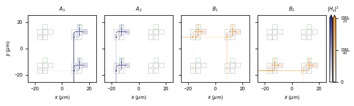
Signal Routing¶

In this section, we illustrate the signal paths along which pulse trains from each port propagate inside the device.

[7]:

from matplotlib.colors import ListedColormap

color_a = (46 / 256, 49 / 256, 146 / 256)
color_b = (247 / 256, 147 / 256, 30 / 256)
cmap_a = ListedColormap(
    1 + np.arange(256).reshape(-1, 1) / 256 * (np.array(color_a) - 1).reshape(1, -1)
)
cmap_b = ListedColormap(
    1 + np.arange(256).reshape(-1, 1) / 256 * (np.array(color_b) - 1).reshape(1, -1)
)


signal = np.array((1, -1, -1, 1))

x, y = field_freq["x"], field_freq["y"]
Hz = field_freq["Hz_center"]
vmax = (np.abs(Hz).max()) ** 2 / 20

fig, ax = plt.subplots(
    1, 4, figsize=(7, 2.1), sharex=True, sharey=True, tight_layout=True
)
ax[0].pcolormesh(
    x, y, np.abs(Hz[0]) ** 2, vmin=0, vmax=vmax, cmap=cmap_a, rasterized=True
)
pca = ax[1].pcolormesh(
    x, y, np.abs(Hz[1]) ** 2, vmin=0, vmax=vmax, cmap=cmap_a, rasterized=True
)
ax[2].pcolormesh(
    x, y, np.abs(Hz[2]) ** 2, vmin=0, vmax=vmax, cmap=cmap_b, rasterized=True
)
pcb = ax[3].pcolormesh(
    x, y, np.abs(Hz[3]) ** 2, vmin=0, vmax=vmax, cmap=cmap_b, rasterized=True
)

ax[0].set(
    xticks=(-20, 0, 20),
    yticks=(-20, 0, 20),
    xlim=(-lattice_const * N_cell[0] / 2, lattice_const * N_cell[0] / 2),
    ylim=(-lattice_const * N_cell[1] / 2, lattice_const * N_cell[1] / 2),
)

x_module = l_des / 2 * np.array([1, 1, -1, -1, 1])
y_module = l_des / 2 * np.array([1, -1, -1, 1, 1])


[
    ax[i].plot(
        x + dist_module + x_module,
        y + y_module,
        color=plt.cm.PRGn(0.2),
        ls="--",
        lw=0.4,
    )
    for x in x_cell_center
    for y in y_cell_center
    for i in range(4)
]
[
    ax[i].plot(
        x + x_module,
        y + dist_module + y_module,
        color=plt.cm.PRGn(0.8),
        ls="--",
        lw=0.4,
    )
    for x in x_cell_center
    for y in y_cell_center
    for i in range(4)
]
[
    ax[i].plot(x - dist_module + x_module, y + y_module, color="gray", ls="--", lw=0.4)
    for x in x_cell_center
    for y in y_cell_center
    for i in range(4)
]
[
    ax[i].plot(x + x_module, y - dist_module + y_module, color="gray", ls="--", lw=0.4)
    for x in x_cell_center
    for y in y_cell_center
    for i in range(4)
]
[
    ax[i].plot(x + x_module, y + y_module, color="gray", ls="--", lw=0.4)
    for x in x_cell_center
    for y in y_cell_center
    for i in range(4)
]
[
    ax[i].plot(
        x - dist_module + x_module,
        y - dist_module + y_module,
        color="gray",
        ls="--",
        lw=0.4,
    )
    for x in x_cell_center
    for y in y_cell_center
    for i in range(4)
]

cbaxs_a = ax[3].inset_axes([1.05, 0, 0.04, 1])
cbar_a = plt.colorbar(pca, cax=cbaxs_a, extend="max")
cbar_a.ax.set_yticks([0, vmax / 2, vmax])
cbar_a.ax.set_yticklabels([])
cbar_a.ax.set_title(r"   $|H_z|^2$", fontsize=7)
cbaxs_b = ax[3].inset_axes([1.1, 0, 0.04, 1])
cbar_b = plt.colorbar(pcb, cax=cbaxs_b, extend="max")
cbar_b.ax.set_yticks([0, vmax / 2, vmax])
cbar_b.ax.set_yticklabels(
    [0, r"$\frac{\mathrm{max}}{40}$", r"$\frac{\mathrm{max}}{20}$"]
)

ax[0].set(xlabel=r"$x$ ($\mu$m)", ylabel=r"$y$ ($\mu$m)")
ax[1].set(xlabel=r"$x$ ($\mu$m)")
ax[2].set(xlabel=r"$x$ ($\mu$m)")
ax[3].set(xlabel=r"$x$ ($\mu$m)")

ax[0].set_title(r"$A_1$", fontsize=7)
ax[1].set_title(r"$A_2$", fontsize=7)
ax[2].set_title(r"$B_1$", fontsize=7)
ax[3].set_title(r"$B_2$", fontsize=7)

[7]:

Text(0.5, 1.0, '$B_2$')

Time-domain Postprocessing¶

Now, using the four base simulations, we define some auxiliary methods to process pulse trains.

env filters out the carrier frequency component, effectively returning the envelope of given signal.
delayed returns $f(t- N_\mathrm{delay}t_\mathrm{delay})$ given $f(t)$ and $N_\mathrm{delay}$.
time_signals returns input and output pulse trains given matrices $A$ and $B$.

Finally, normalizer is a constant matrix $\Delta P$ with $$\Delta P_{i,j} = \int dt [P^C_{ij}(t) - P^D_{ij}(t)],$$ where $P^{C,D}_{ij}$ are the output pulse trains of time signals for $A =[\delta_{1,i}, \delta_{2,i}]$ and $B =[\delta_{1,j}, \delta_{2,j}]$. This is used to normalize power integration values for arbitrary matrix-matrix multiplication.

[8]:

def env(t, signal):
    dt = t[1] - t[0]
    T_period = dt * len(t)
    df = 1 / T_period
    f = df.data * np.arange(len(t))
    FFT_signal = np.fft.fft(signal)
    FFT_signal_filtered = FFT_signal * ((f < freq0) + (f > f[-1] - freq0))
    signal_env = np.fft.ifft(FFT_signal_filtered) * 2
    return np.real(signal_env)


t = thru_flux_time["t"]
dt = t[1] - t[0]
delay_idx = int(t_delay / dt)
t_offset = t[np.argmax(env(t, thru_flux_time["A11"][1]))]


def delayed(signal, N_delay: int = 0, N_pulse: int = 2):
    if N_pulse == 1:
        return signal
    else:
        if len(signal.shape) == 1:
            return np.concat(
                [
                    np.zeros(delay_idx * N_delay),
                    signal,
                    np.zeros(delay_idx * (N_pulse - 1 - N_delay)),
                ]
            )
        else:
            return np.concat(
                [
                    np.zeros([delay_idx * N_delay, *signal.shape[1:]]),
                    signal,
                    np.zeros([delay_idx * (N_pulse - 1 - N_delay), *signal.shape[1:]]),
                ],
                axis=0,
            )


def time_signals(signal_A, signal_B):
    N_pulse = len(signal_A)
    t_ext = dt * np.arange(len(t) + delay_idx * (N_pulse - 1))

    input_signal_A = [
        signal_A[pulse, nx] ** 2
        * delayed(env(t, thru_flux_time[f"A{nx}1"][nx]), N_delay=pulse, N_pulse=N_pulse)
        for pulse in range(N_pulse)
        for nx in range(N_cell[0])
    ]
    input_signal_A = (
        np.array(input_signal_A).reshape(N_pulse, N_cell[0], -1).sum(axis=0)
    )
    input_signal_B = [
        signal_B[pulse, ny] ** 2
        * delayed(
            env(t, thru_flux_time[f"B1{ny}"][N_cell[0] + ny]),
            N_delay=pulse,
            N_pulse=N_pulse,
        )
        for pulse in range(N_pulse)
        for ny in range(N_cell[1])
    ]
    input_signal_B = (
        np.array(input_signal_B).reshape(N_pulse, N_cell[1], -1).sum(axis=0)
    )

    output_signal_C = []
    output_signal_D = []
    output_signal_raw = []

    for nx in range(N_cell[0]):
        for ny in range(N_cell[1]):
            field = det_field_time[f"C{nx}{ny}"]
            field = [
                delayed(
                    np.sum(
                        field
                        * np.concat([signal_A[pulse, :], signal_B[pulse, :]]).reshape(
                            -1, 1, 1, 1
                        ),
                        axis=0,
                    ),
                    N_delay=pulse,
                    N_pulse=N_pulse,
                )
                for pulse in range(N_pulse)
            ]
            field = np.sum(field, axis=0)
            Ex, Ey, Hx, Hy = field[:, 0], field[:, 1], field[:, 2], field[:, 3]
            flux_C = env(t_ext, np.average(Ex * Hy - Ey * Hx, axis=1) * l_des**2)
            output_signal_C.append(flux_C)

            field = det_field_time[f"D{nx}{ny}"]
            field = [
                delayed(
                    np.sum(
                        field
                        * np.concat([signal_A[pulse, :], signal_B[pulse, :]]).reshape(
                            -1, 1, 1, 1
                        ),
                        axis=0,
                    ),
                    N_delay=pulse,
                    N_pulse=N_pulse,
                )
                for pulse in range(N_pulse)
            ]
            field = np.sum(field, axis=0)
            Ex, Ey, Hx, Hy = field[:, 0], field[:, 1], field[:, 2], field[:, 3]
            flux_D = env(t_ext, np.average(Ex * Hy - Ey * Hx, axis=1) * l_des**2)
            output_signal_D.append(flux_D)
            output_signal_raw.append(flux_C - flux_D)

    output_signal_C = np.array(output_signal_C).reshape(2, 2, -1)
    output_signal_D = np.array(output_signal_D).reshape(2, 2, -1)
    output_signal_raw = np.array(output_signal_raw).reshape(2, 2, -1)
    return (
        t_ext,
        (input_signal_A, input_signal_B),
        (output_signal_C, output_signal_D, output_signal_raw),
    )


## Computing normalization value for each cell
normalizer = []
for nx in range(N_cell[0]):
    for ny in range(N_cell[1]):
        sig_A = 0.0 + (np.arange(N_cell[0]) == nx).reshape(1, -1)
        sig_B = 0.0 + (np.arange(N_cell[1]) == ny).reshape(1, -1)
        _, _, (_, _, output_raw) = time_signals(sig_A, sig_B)
        normalizer.append(output_raw[nx, ny])

normalizer = np.array(normalizer).reshape(*N_cell, -1).sum(axis=-1)

Pulse Train Example¶

We now illustrate the input matrices $A, B$ as synchronized pulse trains. Here, the input matrices are randomly generated.

[9]:

N_pulse = 10
np.random.seed(1)
sig_A, sig_B = np.random.uniform(low=-1, high=1, size=(2, N_pulse, 2))

print(r"A = ")
print(sig_A)

print(r"B = ")
print(sig_B)

result_truth = sig_A.T @ sig_B
print("The ground truth result is:")
print(result_truth)

A = 
[[-0.16595599  0.44064899]
 [-0.99977125 -0.39533485]
 [-0.70648822 -0.81532281]
 [-0.62747958 -0.30887855]
 [-0.20646505  0.07763347]
 [-0.16161097  0.370439  ]
 [-0.5910955   0.75623487]
 [-0.94522481  0.34093502]
 [-0.1653904   0.11737966]
 [-0.71922612 -0.60379702]]
B = 
[[ 0.60148914  0.93652315]
 [-0.37315164  0.38464523]
 [ 0.7527783   0.78921333]
 [-0.82991158 -0.92189043]
 [-0.66033916  0.75628501]
 [-0.80330633 -0.15778475]
 [ 0.91577906  0.06633057]
 [ 0.38375423 -0.36896874]
 [ 0.37300186  0.66925134]
 [-0.96342345  0.50028863]]
The ground truth result is:
[[ 0.25551068 -0.81068574]
 [ 1.15518393 -0.3969829 ]]

[10]:

t_ext, inputs, outputs = time_signals(sig_A, sig_B)

color_a = (46 / 256, 49 / 256, 146 / 256)
color_b = (247 / 256, 147 / 256, 30 / 256)
color_c = plt.cm.PRGn(0.9)
color_d = plt.cm.PRGn(0.1)

fig, ax = plt.subplots(4, 2, sharex=True, tight_layout=True, figsize=(4.3, 2.3))

ax[0, 0].plot((t_ext - t_offset) / 1e-12, inputs[0][0], color=color_a, lw=0.75)
ax[1, 0].plot((t_ext - t_offset) / 1e-12, inputs[0][1], color=color_a, lw=0.75)
ax[2, 0].plot((t_ext - t_offset) / 1e-12, inputs[1][0], color=color_b, lw=0.75)
ax[3, 0].plot((t_ext - t_offset) / 1e-12, inputs[1][1], color=color_b, lw=0.75)
ax[0, 0].fill_between(
    (t_ext - t_offset) / 1e-12, inputs[0][0], color=color_a, lw=0.01, alpha=0.2
)
ax[1, 0].fill_between(
    (t_ext - t_offset) / 1e-12, inputs[0][1], color=color_a, lw=0.01, alpha=0.2
)
ax[2, 0].fill_between(
    (t_ext - t_offset) / 1e-12, inputs[1][0], color=color_b, lw=0.01, alpha=0.2
)
ax[3, 0].fill_between(
    (t_ext - t_offset) / 1e-12, inputs[1][1], color=color_b, lw=0.01, alpha=0.2
)

ax[0, 1].plot((t_ext - t_offset) / 1e-12, outputs[0][0, 0], color=color_c, lw=0.75)
ax[1, 1].plot((t_ext - t_offset) / 1e-12, outputs[0][0, 1], color=color_c, lw=0.75)
ax[2, 1].plot((t_ext - t_offset) / 1e-12, outputs[0][1, 0], color=color_c, lw=0.75)
ax[3, 1].plot((t_ext - t_offset) / 1e-12, outputs[0][1, 1], color=color_c, lw=0.75)
ax[0, 1].fill_between(
    (t_ext - t_offset) / 1e-12, outputs[0][0, 0], color=color_c, lw=0.01, alpha=0.2
)
ax[1, 1].fill_between(
    (t_ext - t_offset) / 1e-12, outputs[0][0, 1], color=color_c, lw=0.01, alpha=0.2
)
ax[2, 1].fill_between(
    (t_ext - t_offset) / 1e-12, outputs[0][1, 0], color=color_c, lw=0.01, alpha=0.2
)
ax[3, 1].fill_between(
    (t_ext - t_offset) / 1e-12, outputs[0][1, 1], color=color_c, lw=0.01, alpha=0.2
)

ax[0, 1].plot(
    (t_ext - t_offset) / 1e-12, outputs[1][0, 0], ls="--", color=color_d, lw=0.75
)
ax[1, 1].plot(
    (t_ext - t_offset) / 1e-12, outputs[1][0, 1], ls="--", color=color_d, lw=0.75
)
ax[2, 1].plot(
    (t_ext - t_offset) / 1e-12, outputs[1][1, 0], ls="--", color=color_d, lw=0.75
)
ax[3, 1].plot(
    (t_ext - t_offset) / 1e-12, outputs[1][1, 1], ls="--", color=color_d, lw=0.75
)
ax[0, 1].fill_between(
    (t_ext - t_offset) / 1e-12,
    outputs[1][0, 0],
    ls="--",
    color=color_d,
    lw=0.01,
    alpha=0.2,
)
ax[1, 1].fill_between(
    (t_ext - t_offset) / 1e-12,
    outputs[1][0, 1],
    ls="--",
    color=color_d,
    lw=0.01,
    alpha=0.2,
)
ax[2, 1].fill_between(
    (t_ext - t_offset) / 1e-12,
    outputs[1][1, 0],
    ls="--",
    color=color_d,
    lw=0.01,
    alpha=0.2,
)
ax[3, 1].fill_between(
    (t_ext - t_offset) / 1e-12,
    outputs[1][1, 1],
    ls="--",
    color=color_d,
    lw=0.01,
    alpha=0.2,
)

ax[3, 0].set(xlim=(-0.5, 4.5), xlabel=r"$t$ (ps)")
ax[3, 1].set(xlim=(-0.5, 4.5), xlabel=r"$t$ (ps)")

CD_max = max(outputs[0].max(), outputs[1].max())
[ax[i, 0].set(ylim=(0, 2)) for i in range(4)]
[ax[i, 1].set(ylim=(0, CD_max * 1.1)) for i in range(4)]

ax[0, 0].set(ylabel=r"$P^A_1(t)$")
ax[1, 0].set(ylabel=r"$P^A_2(t)$")
ax[2, 0].set(ylabel=r"$P^B_1(t)$")
ax[3, 0].set(ylabel=r"$P^B_2(t)$")

ax[0, 1].set(ylabel=r"$P^{C,D}_{1,1}(t)$")
ax[1, 1].set(ylabel=r"$P^{C,D}_{1,2}(t)$")
ax[2, 1].set(ylabel=r"$P^{C,D}_{2,1}(t)$")
ax[3, 1].set(ylabel=r"$P^{C,D}_{2,2}(t)$")

result_output = outputs[2].sum(axis=2) / normalizer

for nx in range(2):
    for ny in range(2):
        str_output_c = f"{round(outputs[0][nx, ny].sum() / normalizer[nx, ny], 3)}"
        ax[nx * 2 + ny, 1].text(
            0, 0.5, str_output_c, ha="left", fontsize=6, color=color_c
        )
        str_output_d = f"- {round(outputs[1][nx, ny].sum() / normalizer[nx, ny], 3)}"
        ax[nx * 2 + ny, 1].text(
            0.7, 0.5, str_output_d, ha="left", fontsize=6, color=color_d
        )
        str_output_out = f"= {round(outputs[2][nx, ny].sum() / normalizer[nx, ny], 3)}"
        ax[nx * 2 + ny, 1].text(
            1.55, 0.5, str_output_out, ha="left", fontsize=6, color="k"
        )


[
    ax[i, 0].axvline(x=pulse * t_delay / 1e-12, color="gray", lw=0.5, ls="--")
    for pulse in range(2)
    for i in range(4)
]

ax[0, 0].set_title("Input pulse trains", fontsize=7)
ax[0, 1].set_title("Output pulse trains", fontsize=7)

[ax[i, j].spines["top"].set_visible(False) for i in range(4) for j in range(2)]
[ax[i, j].spines["right"].set_visible(False) for i in range(4) for j in range(2)]

[10]:

[None, None, None, None, None, None, None, None]

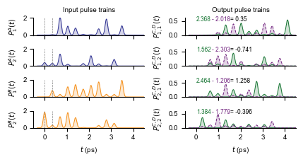
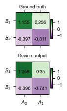
Multiplication Result¶

In this section, we compare the ground truth result for multiplication $A^T B$ and the corresponding device output result. The device output is obtained by the difference in time integration of power envelopes for detectors $C$ and $D$, followed by normalization with normalizer.

[11]:

fig, ax = plt.subplots(
    2, 1, sharex=True, sharey=True, tight_layout=True, figsize=(1.3, 2.3)
)
ax[0].matshow(result_truth[::-1].T, vmin=-1.5, vmax=1.5, cmap=plt.cm.PRGn)
ms = ax[1].matshow(result_output[::-1].T, vmin=-1.5, vmax=1.5, cmap=plt.cm.PRGn)

[
    ax[0].text(n, m, round(result_truth[::-1].T[m, n], 3), va="top", ha="center")
    for m in range(2)
    for n in range(2)
]
[
    ax[1].text(n, m, round(result_output[::-1].T[m, n], 3), va="top", ha="center")
    for m in range(2)
    for n in range(2)
]

# ax[0].xaxis.set_ticks_position('bottom')
ax[1].xaxis.set_ticks_position("bottom")

ax[1].set(xticks=(0, 1), xticklabels=[r"$A_2$", r"$A_1$"])
ax[1].set(yticks=(1, 0), yticklabels=[r"$B_2$", r"$B_1$"])
ax[0].set(yticks=(1, 0), yticklabels=[r"$B_2$", r"$B_1$"])

cax0 = ax[0].inset_axes([1.05, 0.2, 0.05, 0.6])
cax1 = ax[1].inset_axes([1.05, 0.2, 0.05, 0.6])
cbar = plt.colorbar(ms, cax=cax0)
cbar = plt.colorbar(ms, cax=cax1)

ax[0].set_title("Ground truth", fontsize=7)
ax[1].set_title("Device output", fontsize=7)

[11]:

Text(0.5, 1.0, 'Device output')

TIDY3D
LEARNING CENTER

Photonic systolic array for all-optical matrix-matrix multiplication¶

Define Simulation¶

Run Simulations¶

Data Loading¶

Signal Routing¶

Time-domain Postprocessing¶

Pulse Train Example¶

Multiplication Result¶

More Notebooks

TIDY3D LEARNING CENTER

Photonic systolic array for all-optical matrix-matrix multiplication¶

Define Simulation¶

Run Simulations¶

Data Loading¶

Signal Routing¶

Time-domain Postprocessing¶

Pulse Train Example¶

Multiplication Result¶

More Notebooks

TIDY3D
LEARNING CENTER