Author: Guodong Zhu, Vanderbilt University

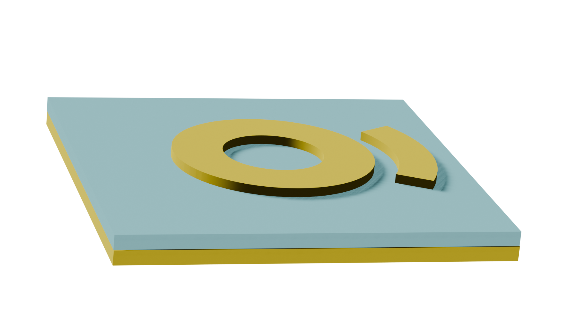
In this notebook, we simulate a high-Q-factor plasmonic thermal emitter utilizing surface lattice resonance. By adjusting the design of periodic nanostructures, sharp resonance modes can be supported, resulting in enhanced and spectrally selective thermal emission.

The model consists of a unit cell with periodic boundary conditions. Absorption is calculated under plane wave illumination. According to Kirchhoff’s law, emission equals absorption at thermal equilibrium, allowing us to use the absorption results to determine the thermal emission properties of the structure.

[1]:

import matplotlib.pylab as plt
import numpy as np

import tidy3d as td
import tidy3d.web as web

Simulation Setup¶

[2]:

# units definitions
um = 1e0
nm = 1e-3
wavelength = 4.0  # center wavelength

Since the simulations might involve resonances, a relatively long runtime is set.

[3]:

wavelengths = np.linspace(wavelength - 1 * um, wavelength + 1 * um, 1001)
freqs = td.C_0 / wavelengths
freq0 = (np.max(freqs) + np.min(freqs)) / 2.0  # center frequency
fwidth = np.max(freqs) - np.min(freqs)
run_time = 5e-11

[4]:

# defining mediums
medium_Al2O3 = td.Medium(permittivity=1.685**2)
medium_gold = td.material_library["Au"]["Olmon2012evaporated"]
medium_air = td.Medium(permittivity=1**2)

[5]:

size_design_x = 4000 * nm
size_design_y = 4000 * nm
thick_metal = 100 * nm
thick_spacer = 0.15
thick_reflector = 0.15
thick_sub = 8.0 - thick_spacer - thick_reflector
thick_air = 8.0 - thick_metal

mask_radius = 1690 * nm
size_x = size_design_x
size_y = size_design_y
size_z = thick_sub + thick_metal + thick_air + thick_spacer + thick_reflector
top_z = size_z / 2.0

center_metal_z = top_z - thick_air - thick_metal / 2.0
center_spacer_z = top_z - thick_air - thick_metal - thick_spacer / 2.0
center_reflector_z = (
    top_z - thick_air - thick_metal - thick_spacer - thick_reflector / 2.0
)

Auxiliary function to define the geometry.

[6]:

def sector_vertices(x0, y0, R, n, theta):
    vertices = []
    vertices.append((x0, y0))

    for i in range(n, 0, -1):
        theta_i = i * theta / n
        Xp = x0 + R * np.cos(theta_i)
        Yp = y0 + R * np.sin(theta_i)
        vertices.append((Xp, Yp))
    for i in range(0, n + 1, 1):
        theta_i = -i * theta / n
        Xp = x0 + R * np.cos(theta_i)
        Yp = y0 + R * np.sin(theta_i)
        vertices.append((Xp, Yp))

    return vertices

Next, we create an auxiliary function to return the Simulation object as a function of the incident angle. Note that we will use a FixedAngleSpec for the PlaneWave angular_spec argument, which ensures that the same angle is fixed for the entire source spectrum. A more detailed discussion can be found here.

Due to geometric features that are much smaller than the wavelength, we will also add a MeshOverrideStructure region to locally refine the mesh and correctly resolve the geometry.

Due to resonant effects and to reduce computational cost, we will reduce the default simulation shutoff to $10^{-4}$.

[7]:

def make_sim(
    polarization_angle: float,
    incident_angle: float = 0,
    outerR: float = 1.68,
    innerR: float = 1.04,
) -> td.Simulation:
    # structures
    sector = td.Structure(
        geometry=td.PolySlab(
            vertices=sector_vertices(0, 0, outerR, 20, np.deg2rad(30)),
            axis=2,
            slab_bounds=(0, thick_metal),
        ),
        medium=medium_gold,
    )
    cylinder_air_2 = td.Structure(
        geometry=td.Cylinder(
            axis=2,
            radius=1.29,
            center=(0, 0, thick_metal / 2.0),
            length=thick_metal,
        ),
        medium=medium_air,
    )
    cylinder = td.Structure(
        geometry=td.Cylinder(
            axis=2,
            radius=innerR,
            center=(0, 0, thick_metal / 2.0),
            length=thick_metal,
        ),
        medium=medium_gold,
    )

    cylinder_air = td.Structure(
        geometry=td.Cylinder(
            axis=2,
            radius=innerR / 2.0,
            center=(0, 0, thick_metal / 2.0),
            length=thick_metal,
        ),
        medium=medium_air,
    )

    spacer = td.Structure(
        geometry=td.Box.from_bounds(
            rmin=(-td.inf, -td.inf, center_spacer_z - thick_spacer / 2.0),
            rmax=(+td.inf, +td.inf, center_spacer_z + thick_spacer / 2.0),
        ),
        medium=medium_Al2O3,
    )

    reflector = td.Structure(
        geometry=td.Box.from_bounds(
            rmin=(-td.inf, -td.inf, center_reflector_z - thick_reflector / 2.0),
            rmax=(+td.inf, +td.inf, center_reflector_z + thick_reflector / 2.0),
        ),
        medium=medium_gold,
    )

    substrate = td.Structure(
        geometry=td.Box(
            center=(0, 0, -size_z + thick_sub),
            size=(td.inf, td.inf, size_z),
        ),
        medium=medium_Al2O3,
    )

    # plane wave source
    plane_wave = td.PlaneWave(
        center=(0, 0, size_z / 2 - 2),
        size=(td.inf, td.inf, 0),
        source_time=td.GaussianPulse(freq0=freq0, fwidth=fwidth),
        pol_angle=polarization_angle,
        angle_theta=incident_angle,
        direction="-",
        angular_spec=td.FixedAngleSpec(),
    )

    # monitors
    reflection = td.FluxMonitor(
        center=(0, 0, size_z / 2 - 1),
        size=(td.inf, td.inf, 0),
        freqs=freqs,
        name="reflection",
    )

    transmission = td.FluxMonitor(
        center=(0, 0, -size_z / 2 + 1),
        size=(td.inf, td.inf, 0),
        freqs=freqs,
        name="transmission",
    )

    # mesh refinement
    mesh_overrides = [
        td.MeshOverrideStructure(
            geometry=td.Box.from_bounds(
                rmin=(-td.inf, -td.inf, center_reflector_z - thick_reflector / 2.0),
                rmax=(+td.inf, +td.inf, center_metal_z + thick_metal / 2.0),
            ),
            dl=[80 * nm, 80 * nm, 20 * nm],
        )
    ]

    my_sim = td.Simulation(
        size=(size_x, size_y, size_z),
        run_time=run_time,
        structures=[
            substrate,
            spacer,
            reflector,
            sector,
            cylinder_air_2,
            cylinder,
            cylinder_air,
        ],
        sources=[plane_wave],
        monitors=[reflection, transmission],
        boundary_spec=td.BoundarySpec(
            x=td.Boundary.periodic(),
            y=td.Boundary.periodic(),
            z=td.Boundary(plus=td.PML(), minus=td.Absorber(num_layers=80)),
        ),
        grid_spec=td.GridSpec.auto(
            wavelength=wavelength,
            min_steps_per_wvl=20,
            override_structures=mesh_overrides,
        ),
        medium=medium_air,
        shutoff=1e-4,
    )
    return my_sim

[8]:

sim = make_sim(np.deg2rad(0.0), np.deg2rad(0.0), 1.68, 1.04)

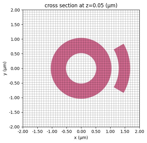
Next, we plot the grid to ensure that the structure is properly resolved by the mesh.

[9]:

ax = sim.plot(z=center_metal_z)
sim.plot_grid(z=center_metal_z, ax=ax)
plt.show()

No description has been provided for this image

Postprocessing¶

[10]:

sim_data = td.web.run(sim, task_name="simulation_at_normal_incident", verbose=True)

17:19:43 -03 Created task 'simulation_at_normal_incident' with task_id          
             'fdve-ff872fab-3c73-424d-a648-46f2149ba891' and task_type 'FDTD'.

             View task using web UI at                                          
             'https://tidy3d.simulation.cloud/workbench?taskId=fdve-ff872fab-3c7
             3-424d-a648-46f2149ba891'.

             Task folder: 'default'.

Output()

17:19:46 -03 Maximum FlexCredit cost: 0.212. Minimum cost depends on task       
             execution details. Use 'web.real_cost(task_id)' to get the billed  
             FlexCredit cost after a simulation run.

17:19:47 -03 status = success

Output()

17:19:49 -03 loading simulation from simulation_data.hdf5

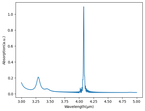
We can calculate the absorption using the relation $1 = A + R + T$, where $A$ is the absorption, $R$ is the reflection, and $T$ is the transmission.

A strong absorption peak can be seen around 4.1 µm.

[11]:

R = sim_data["reflection"].flux
T = abs(sim_data["transmission"].flux)
plt.plot(wavelengths, 1 - (R + T))
plt.xlabel("Wavelength(µm)")
plt.ylabel("Absorption(a.u.)")
plt.show()

Band Structure¶

Next, we run a Batch of simulations, varying the incident angle to analyze the angular emission.

[12]:

angle_list = np.linspace(0, 6, 11)  # theta values for the parameter sweep
# create a dictionary of simulations
sims = {
    f"theta={theta:.1f}": make_sim(np.deg2rad(0), np.deg2rad(theta), 1.68, 1.04)
    for theta in angle_list
}

# create and run a batch of simulations
batch = web.Batch(simulations=sims, folder_name="sweep_angle_ring")
batch.estimate_cost()

17:20:30 -03 Maximum FlexCredit cost: 6.943 for the whole batch.

[12]:

6.9431660107445525

[13]:

batch_results = batch.run(path_dir="sweep_angle_ring")

Output()

             Started working on Batch containing 11 tasks.

17:20:43 -03 Maximum FlexCredit cost: 6.943 for the whole batch.

             Use 'Batch.real_cost()' to get the billed FlexCredit cost after the
             Batch has completed.

Output()

17:20:52 -03 Batch complete.

Output()

After running, we can check the real billed cost for the whole batch.

[14]:

batch.real_cost()

17:21:06 -03 Total billed flex credit cost: 8.912.

[14]:

8.91216872032322

[15]:

td.config.logging_level = "ERROR"

R = np.array(
    [
        np.abs(batch_results[f"theta={theta:.1f}"]["reflection"].flux.values)
        for theta in angle_list
    ]
)

T = np.array(
    [
        np.abs(batch_results[f"theta={theta:.1f}"]["transmission"].flux.values)
        for theta in angle_list
    ]
)

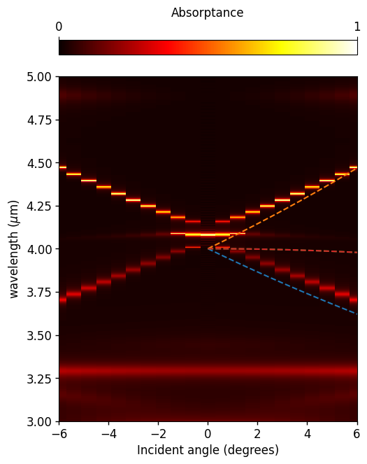
Finally, we can visualize the absorption as a function of the incident angle and compare it with the diffraction results. This allows us to see how the structure’s resonances relate to the underlying lattice diffraction conditions and to distinguish between purely geometric diffraction features and true surface lattice resonances.

[16]:

Absorption_matrix = 1.0 - (T + R)

fig, ax1 = plt.subplots(figsize=(5.5, 8))
absorption_all = np.concatenate((Absorption_matrix[::-1, :], Absorption_matrix), axis=0)
theta_list_all = np.concatenate((-angle_list[::-1], angle_list), axis=0)
ks = np.sin(np.deg2rad(theta_list_all))
im = ax1.pcolormesh(
    theta_list_all, td.C_0 / freqs, absorption_all.T, cmap="hot", vmin=0, vmax=1
)
ax1.set_xlabel("Incident angle (degrees)", fontsize=12)
ax1.set_xlim([-6, 6])
ax1.set_ylim([3, 5])
ax1.set_ylabel(r"wavelength ($\mu$m)", fontsize=12)
ax1.tick_params(width=1, labelsize=12)
cbar = plt.colorbar(im, pad=0.05, orientation="horizontal", location="top")
cbar.set_ticks([0.0, 1.0])
cbar.ax.tick_params(labelsize=12)
cbar.set_label("Absorptance", fontsize=12)
cbar.ax.tick_params(labelsize=12)

# Constants
c = td.C_0  # speed of light [um/s]
Px = 4.0  # lattice period in x [um]
Py = 4.0  # lattice period in y [um]

# Diffraction orders
orders = np.array(
    [
        [1, 0],
        [-1, 0],
        [0, 1],
        [0, -1],
    ]
)

# Normalized kx values
kx_norm = np.linspace(0, 0.5, 500)
theta_k = np.rad2deg(np.arcsin(kx_norm))
for p, q in orders:
    f = np.sqrt(
        (kx_norm * 2 * np.pi / Px + p * 2 * np.pi / Px) ** 2 + (q * 2 * np.pi / Py) ** 2
    )
    kx = 2 * np.pi * kx_norm / Px
    wavelengths = 2 * np.pi / f

    ax1.plot(theta_k, wavelengths, "--", label=f"({p},{q})")

plt.show()