Author: Dr. Judson Ryckman, Clemson University
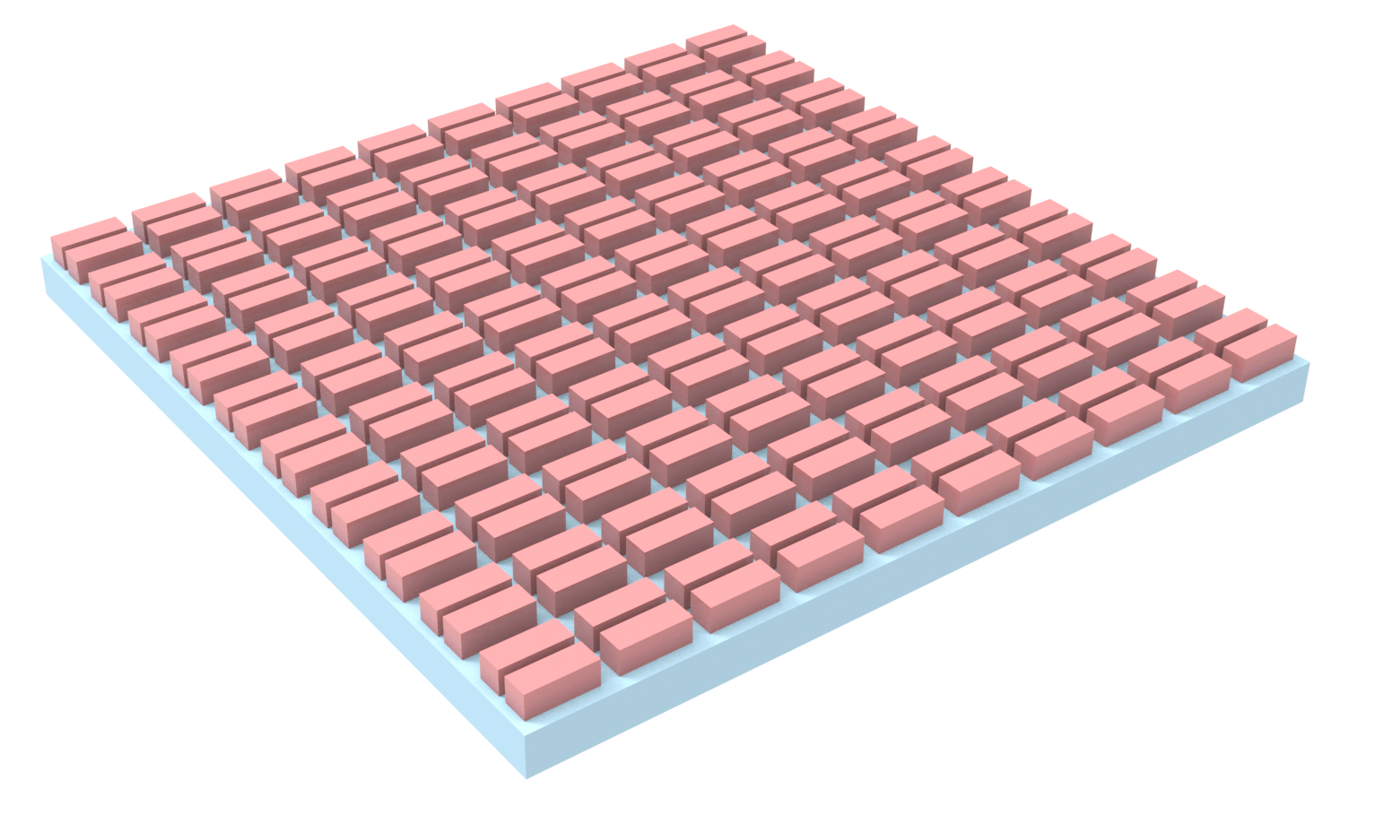
This notebook builds a pSi square-grating guided-mode-resonance (GMR) reflector in Tidy3D, visualizes the geometry, runs a cloud simulation, and plots the reflection spectrum.
Notes:
- This model allows for simulation of an anisotropic material in the core and cladding using either a non-dispersive, user specified material, or a pre-fitted dispersive material model.
This notebook is associated with the publication T. Dash, S. Gafsi, E. M. Dos Santos, I. Kravchenko, and J. D. Ryckman, “Responsive Visible-Wavelength Metasurfaces from Porous Silicon Based on Fano Guided-Mode Resonance.” Adv. Optical Mater. (2025): e02295. DOI: 10.1002/adom.202502295.
[1]:
import matplotlib.pyplot as plt
import numpy as np
import tidy3d as td
import tidy3d.web as web
[2]:
# Define geometry (microns)
period = 0.5
wl_min = 0.4
wl_max = 0.8
size_z = 3
gap = 0.15
slab_thick = 0.09
etch_depth = 0.15
cd_bias = 0.045
duty_cycle = 0.5 + cd_bias / period
[3]:
use_dispersive_material_model = True  # True or False

# If using non-dispersive model
n_core = 1.54
n_clad = 1.19
delta_n = 0.05
k_core = 0.005

# Define background medium
Vacuum = td.Medium(
    name="Vacuum",
)
[4]:
# Define anisotropic materials (dispersive or non-dispersive)

if use_dispersive_material_model:
    # --- Dispersive material model ---
    anisotropic_cladding = td.AnisotropicMedium(
        name="anisotropic_cladding",
        xx=td.PoleResidue(
            name="clad_ORD_p78_sp65_sigma45",
            frequency_range=[374740572500000, 749481145000000],
            eps_inf=1.285763200610988,
            poles=[
                [
                    (-80006430873749.78 - 3992826532935084.5j),
                    (43225975831.18877 + 65698194005.3712j),
                ],
                [
                    (-254779968980075.38 - 6210018855903866j),
                    (26447240584513.562 + 322970863925251.1j),
                ],
            ],
        ),
        yy=td.PoleResidue(
            name="clad_ORD_p78_sp65_sigma45",
            frequency_range=[374740572500000, 749481145000000],
            eps_inf=1.285763200610988,
            poles=[
                [
                    (-80006430873749.78 - 3992826532935084.5j),
                    (43225975831.18877 + 65698194005.3712j),
                ],
                [
                    (-254779968980075.38 - 6210018855903866j),
                    (26447240584513.562 + 322970863925251.1j),
                ],
            ],
        ),
        zz=td.PoleResidue(
            name="clad_EXT_p78_sp65_sigma45",
            frequency_range=[374740572500000, 749481145000000],
            eps_inf=1.3638432159648597,
            poles=[
                [
                    (-225020803639667.75 - 5894420287418583j),
                    (40348009572759.95 + 529332098674452.8j),
                ],
                [
                    (-70804109316383.19 - 4024765445948748.5j),
                    (49573077608.54553 + 214392902555.40454j),
                ],
                [
                    (-31856302596180.74 - 4185043474496780.5j),
                    (17457996399.55387 - 11843520333.727072j),
                ],
            ],
        ),
    )

    anisotropic_core = td.AnisotropicMedium(
        name="anisotropic_core",
        xx=td.PoleResidue(
            name="core_ORD_p60_sp50_sigma18",
            frequency_range=[374740572500000, 749481145000000],
            eps_inf=1.7636879320933365,
            poles=[
                [
                    (-209812302659551.34 - 5713050507260843j),
                    (91645423757352.25 + 1245780204707888.5j),
                ],
                [
                    (-33767895447480.945 - 4076300334074186.5j),
                    (-383042439354.49066 + 74306357834.59213j),
                ],
                [
                    (-118113417687026.97 - 4102291974502630.5j),
                    (433192944675.4037 + 920226300587.0059j),
                ],
            ],
        ),
        yy=td.PoleResidue(
            name="core_ORD_p60_sp50_sigma18",
            frequency_range=[374740572500000, 749481145000000],
            eps_inf=1.7636879320933365,
            poles=[
                [
                    (-209812302659551.34 - 5713050507260843j),
                    (91645423757352.25 + 1245780204707888.5j),
                ],
                [
                    (-33767895447480.945 - 4076300334074186.5j),
                    (-383042439354.49066 + 74306357834.59213j),
                ],
                [
                    (-118113417687026.97 - 4102291974502630.5j),
                    (433192944675.4037 + 920226300587.0059j),
                ],
            ],
        ),
        zz=td.PoleResidue(
            name="core_EXT_p60_sp50_sigma18",
            frequency_range=[374740572500000, 749481145000000],
            eps_inf=1.8442541496138387,
            poles=[
                [
                    (-194036164426216.44 - 5575364239486789j),
                    (104804935602979.1 + 1468449074428882j),
                ],
                [
                    (-139501019944869.6 - 4570504481783418j),
                    (-1034474504270.1329 - 626357243110.9268j),
                ],
                [
                    (-47718826616363.5 - 4342881289958674.5j),
                    (-370871032855.6184 + 122560276380.73393j),
                ],
                [
                    (-19150839534338.004 - 3934925705165841j),
                    (-2319448769.6423297 - 85365662359.27574j),
                ],
                [
                    (-53127023418600.734 - 4039267182350066j),
                    (-169960900226.993 + 815175929541.1998j),
                ],
            ],
        ),
    )

else:
    # --- Non-dispersive material model ---
    anisotropic_cladding = td.FullyAnisotropicMedium(
        name="anisotropic_cladding",
        permittivity=[
            [n_clad**2 - k_core**2, 0, 0],
            [0, n_clad**2 - k_core**2, 0],
            [0, 0, (n_clad + delta_n) ** 2 - k_core**2],
        ],
        conductivity=[
            [0.0526 * n_clad * k_core, 0, 0],
            [0, 0.0526 * n_clad * k_core, 0],
            [0, 0, 0.0526 * (n_clad + delta_n) * k_core],
        ],
    )

    anisotropic_core = td.FullyAnisotropicMedium(
        name="anisotropic_core",
        permittivity=[
            [n_core**2 - k_core**2, 0, 0],
            [0, n_core**2 - k_core**2, 0],
            [0, 0, (n_core + delta_n) ** 2 - k_core**2],
        ],
        conductivity=[
            [0.0526 * n_core * k_core, 0, 0],
            [0, 0.0526 * n_core * k_core, 0],
            [0, 0, 0.0526 * (n_core + delta_n) * k_core],
        ],
    )
[5]:
# Define frequency and wavelength range
lda0 = 0.6
freq0 = td.C_0 / lda0
ldas = np.linspace(0.4, 0.8, 701)
freqs = td.C_0 / ldas
fwidth = 0.5 * (np.max(freqs) - np.min(freqs))

# Add source
plane_wave = td.PlaneWave(
    name="plane_wave",
    center=[0, 0, size_z / 2 - wl_max / 2],
    size=[td.inf, td.inf, 0],
    source_time=td.GaussianPulse(
        freq0=freq0,
        fwidth=fwidth,
    ),
    direction="-",
)

# Add monitors
Reflection = td.FluxMonitor(
    name="Reflection",
    center=[0, 0, size_z / 2 - wl_max / 4],
    size=[100, 100, 0],
    freqs=freqs,
)

field_XZ = td.FieldMonitor(name="field_XZ", size=[period, 0, size_z], freqs=freqs[::5])

field_YZ = td.FieldMonitor(name="field_YZ", size=[0, period, size_z], freqs=freqs[::5])
[6]:
# Define structures
substrate = td.Structure(
    name="substrate",
    geometry=td.Box(center=[0, 0, -500], size=[2000, 2000, 1000]),
    medium=anisotropic_cladding,
)

core_slab = td.Structure(
    name="core_slab",
    geometry=td.Box(center=[0, 0, slab_thick / 2], size=[5, 5, slab_thick]),
    medium=anisotropic_core,
)

temp_pillar = td.Structure(
    name="temp_pillar",
    geometry=td.Box(
        center=[0, 0, slab_thick / 2],
        size=[period * duty_cycle, period * duty_cycle, slab_thick],
    ),
    medium=anisotropic_cladding,
)

cylinder_N = td.Structure(
    geometry=td.Cylinder(
        axis=0,
        radius=slab_thick,
        center=[0, period * duty_cycle / 2, slab_thick],
        length=duty_cycle * period,
    ),
    name="cylinder_N",
    medium=anisotropic_core,
)

cylinder_S = td.Structure(
    geometry=td.Cylinder(
        axis=0,
        radius=slab_thick,
        center=[0, -period * duty_cycle / 2, slab_thick],
        length=duty_cycle * period,
    ),
    name="cylinder_S",
    medium=anisotropic_core,
)

cylinder_E = td.Structure(
    geometry=td.Cylinder(
        axis=1,
        radius=slab_thick,
        center=[period * duty_cycle / 2, 0, slab_thick],
        length=duty_cycle * period,
    ),
    name="cylinder_E",
    medium=anisotropic_core,
)

cylinder_W = td.Structure(
    geometry=td.Cylinder(
        axis=1,
        radius=slab_thick,
        center=[-period * duty_cycle / 2, 0, slab_thick],
        length=duty_cycle * period,
    ),
    name="cylinder_W",
    medium=anisotropic_core,
)

temp_pillar_slab = td.Structure(
    name="temp_pillar_slab",
    geometry=td.Box(
        center=[0, 0, slab_thick + etch_depth / 2], size=[5, 5, etch_depth]
    ),
    medium=Vacuum,
)

core_pillar = td.Structure(
    name="core_pillar",
    geometry=td.Box(
        center=[0, 0, slab_thick + etch_depth / 2],
        size=[period * duty_cycle, period * duty_cycle, etch_depth],
    ),
    medium=anisotropic_core,
)

internal_pillar = td.Structure(
    name="internal_pillar",
    geometry=td.Box(
        center=[0, 0, slab_thick + etch_depth / 2 - slab_thick],
        size=[
            (period * duty_cycle - 2 * slab_thick)
            * ((period * duty_cycle - 2 * slab_thick) > 0),
            (period * duty_cycle - 2 * slab_thick)
            * ((period * duty_cycle - 2 * slab_thick) > 0),
            etch_depth,
        ],
    ),
    medium=anisotropic_cladding,
)

pillar_cap = td.Structure(
    name="pillar_cap",
    geometry=td.Box(
        center=[0, 0, slab_thick + etch_depth + 0.3], size=[period * 4, period * 4, 0.6]
    ),
    medium=Vacuum,
)
[7]:
# Build simulation
sim = td.Simulation(
    size=[0.5, 0.5, 3],
    boundary_spec=td.BoundarySpec(
        x=td.Boundary.periodic(), y=td.Boundary.periodic(), z=td.Boundary.pml()
    ),
    grid_spec=td.GridSpec.auto(min_steps_per_wvl=24, wavelength=np.min(ldas)),
    shutoff=1e-8,
    run_time=5e-12,
    medium=Vacuum,
    sources=[plane_wave],
    monitors=[Reflection, field_XZ, field_YZ],
    structures=[
        substrate,
        core_slab,
        temp_pillar,
        cylinder_N,
        cylinder_S,
        cylinder_E,
        cylinder_W,
        temp_pillar_slab,
        core_pillar,
        internal_pillar,
        pillar_cap,
    ],
)
[8]:
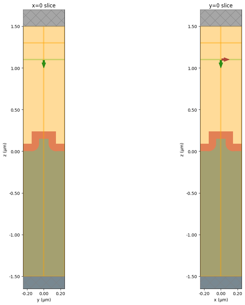
# Visualize 2D cross sections of device geometry
fig, (ax1, ax2) = plt.subplots(1, 2, figsize=(15, 10))
sim.plot(x=0.0, ax=ax1)
ax1.set_title("x=0 slice")
# sim.plot_grid(x=0, ax=ax1) # Optional to inspect grid
sim.plot(y=0.0, ax=ax2)
ax2.set_title("y=0 slice")
# sim.plot_grid(y=0, ax=ax2) # Optional to inspect grid
plt.tight_layout()
plt.show()
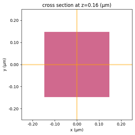
ax3 = sim.plot(z=slab_thick + etch_depth / 2)
# sim.plot_grid(x=0, ax=ax)
plt.show()
[9]:
# Visualize simulation in 3D
sim.plot_3d()
[10]:
# Run the simulation
sim_data = web.run(
    sim,
    task_name="curved_pSi_GMR_Dispersive_Anisotropic_FIG2_FDTD",
    path="./data/sim_data.hdf5",
)
10:43:09 Eastern Daylight Time Created task
                               'curved_pSi_GMR_Dispersive_Anisotropic_FIG2_FDTD'
                               with task_id
                               'fdve-73d81855-284a-498e-9cbc-73546516497d' and
                               task_type 'FDTD'.
                               View task using web UI at
                               'https://tidy3d.simulation.cloud/workbench?taskId
                               =fdve-73d81855-284a-498e-9cbc-73546516497d'.
Task folder: 'default'.
Output()
10:43:11 Eastern Daylight Time Maximum FlexCredit cost: 0.333. Minimum cost
                               depends on task execution details. Use
                               'web.real_cost(task_id)' to get the billed
                               FlexCredit cost after a simulation run.
status = queued
                               To cancel the simulation, use
                               'web.abort(task_id)' or 'web.delete(task_id)' or
                               abort/delete the task in the web UI. Terminating
                               the Python script will not stop the job running
                               on the cloud.
Output()
10:43:18 Eastern Daylight Time starting up solver
running solver
Output()
10:44:29 Eastern Daylight Time early shutoff detected at 44%, exiting.
status = postprocess
Output()
10:44:35 Eastern Daylight Time status = success
10:44:37 Eastern Daylight Time View simulation result at
                               'https://tidy3d.simulation.cloud/workbench?taskId
                               =fdve-73d81855-284a-498e-9cbc-73546516497d'.
Output()
10:44:43 Eastern Daylight Time loading simulation from ./data/sim_data.hdf5
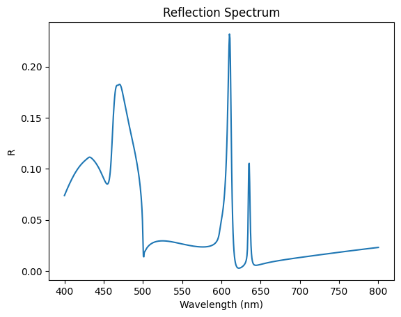
[11]:
# Select reflection monitor by its name in your sim
plot_data = sim_data[
    "Reflection"
].flux  # Adjust "Reflection" if your monitor has a different name

flux_vals = np.abs(plot_data.values)

plt.figure()
plt.plot(ldas * 1e3, flux_vals)
plt.xlabel("Wavelength (nm)")
plt.ylabel("R")
plt.title("Reflection Spectrum")
# plt.gca().invert_xaxis()  # optional: decreasing wavelength left-to-right
plt.show()
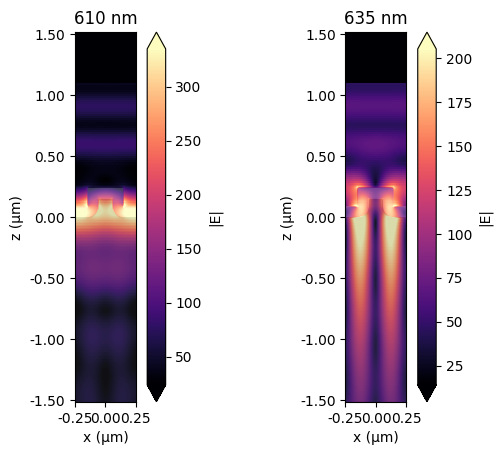
[12]:
# Plot field distributions at the resonances at around 610 nm and 635 nm for example
fig, ax = plt.subplots(1, 2)
idx = np.abs(ldas - 0.61).argmin()
sim_data.plot_field("field_XZ", "E", "abs", f=freqs[idx], ax=ax[0])
ax[0].set_title("610 nm")

idx = np.abs(ldas - 0.635).argmin()
sim_data.plot_field("field_XZ", "E", "abs", f=freqs[idx], ax=ax[1])
ax[1].set_title("635 nm")
plt.show()
[ ]: