


In this notebook, we will demonstrate how to use Tidy3D to simulate a simple RF antenna and compute key antenna metrics, such as:
- S-parameters
- Impedance
- Field profile
- Directivity and Gain
- Axial Ratio
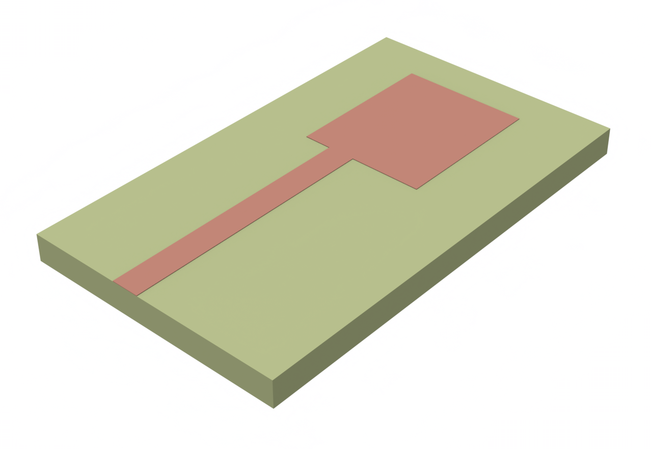
We will use the patch antenna model designed by Sheen et al. in Reference [1]. A rectangular patch antenna is a type of microstrip antenna consisting of a rectangular conductive patch placed on a dielectric substrate with a ground plane on the opposite side. These antennas are widely used in wireless communication applications due to their simple design, ease of fabrication, and low profile.
# Importing necessary libraries
import matplotlib.colors as colors
import matplotlib.pyplot as plt
import numpy as np
import tidy3d as td
import tidy3d.rf as rf
import tidy3d.web as web
Building the Model
Units and Frequency Settings
The antenna has a primary resonance at f ~ 7.5 GHz and a secondary resonance near f ~ 10 GHz. We will choose a frequency range that encompasses both resonances.
# Frequency and wavelength parameters
freq_start = 5e9
freq_stop = 11e9
freq0 = (freq_start + freq_stop) / 2
wavelength0 = td.C_0 / freq0

# Target frequencies (also used to define field monitors)
freqs_target = [7.5e9, 10e9]

# Frequency sweep points
freqs = np.linspace(freq_start, freq_stop, 201)
In Tidy3D, the default units are micrometers (µm) and Hertz (Hz). For convenience during setup, we introduce a scaling factor to convert to millimeters (mm), which is more commonly used in RF simulations.
# Scaling used for millimeters
mm = 1e3
Materials
The dielectric substrate has a constant relative permittivity of 2.2. The metal structures are represented by the perfect electric conductor (PEC) medium.
# Materials present
medium_air = td.Medium(permittivity=1.0, name="Air")
medium_sub = td.Medium(permittivity=2.2, name="Substrate")
medium_metal = td.PECMedium()
Geometry and Structures
We follow the dimensions outlined in Reference [1] to create the patch antenna.
# Metal thickness
th = 0.05 * mm

# Substrate parameters
sub_x = 23.34 * mm
sub_y = 40 * mm
sub_z = 0.794 * mm

# Patch parameters
patch_x = 12.45 * mm
patch_y = 16 * mm

# Feed line parameters
feed_x = 2.46 * mm
feed_y = 20 * mm
feed_offset = 2.09 * mm
The structures are created below.
# Create substrate
substrate = td.Structure(
    geometry=td.Box(center=[0, 0, 0], size=[sub_x, sub_y, sub_z]),
    medium=medium_sub,
    name="Substrate",
)

# Create ground plane
ground_plane = td.Structure(
    geometry=td.Box(center=[0, 0, -(sub_z + th) / 2], size=[sub_x, sub_y, th]),
    medium=medium_metal,
    name="Ground",
)

# Create feed line
feed_line = td.Structure(
    geometry=td.Box.from_bounds(
        rmin=[-patch_x / 2 + feed_offset, -sub_y / 2, sub_z / 2],
        rmax=[-patch_x / 2 + feed_offset + feed_x, -sub_y / 2 + feed_y, sub_z / 2 + th],
    ),
    medium=medium_metal,
    name="Feed line",
)

# Create patch antenna
patch = td.Structure(
    geometry=td.Box.from_bounds(
        rmin=[-patch_x / 2, -sub_y / 2 + feed_y, sub_z / 2],
        rmax=[patch_x / 2, -sub_y / 2 + feed_y + patch_y, sub_z / 2 + th],
    ),
    medium=medium_metal,
    name="Patch",
)
The structures are consolidated into a list below. For best results, we recommend adding any dielectric structures first, followed by metal/PEC structures. This ensures that the metal/PEC overrides the dielectric at the applicable material boundaries.
# List of structures for the simulations
structures_list = [substrate, ground_plane, feed_line, patch]
Monitors
We define a FieldMonitor to observe the field distribution in the patch antenna plane.
# Field monitor to view the electromagnetic fields in the patch plane
monitor_field = td.FieldMonitor(
    center=(0, 0, sub_z / 2),
    size=(td.inf, td.inf, 0),
    freqs=freqs_target,
    name="field",
)
To obtain radiation characteristics such as directivity and gain, use a DirectivityMonitor. The DirectivityMonitor is set up to surround the entire radiating structure and automatically calculates far-field information through a near-to-far field transformation.
# Define elevation and azimuthal angular observation points
# Theta is the elevation angle and defined relative to global +z axis
theta = np.linspace(0, np.pi, 101)
# Phi is the azimuthal angle and defined relative to global +x axis
phi = np.linspace(-np.pi, np.pi, 201)

# Create the DirectivityMonitor
monitor_directivity = rf.DirectivityMonitor(
    center=(0, 0, 0),
    size=(
        30 * mm,
        45 * mm,
        4 * mm,
    ),  # The monitor should enclose the whole structure of interest
    freqs=freqs,
    name="radiation",
    phi=phi,
    theta=theta,
)
11:00:20 EST WARNING: ℹ️ ⚠️ RF simulations are subject to new license requirements
             in the future. You have instantiated at least one RF-specific
             component.
Boundaries
The simulation is truncated by Perfectly Matched Layers (PMLs) on all sides to absorb the outgoing radiation. Additionally, we introduce air padding of approximately half wavelength thickness around the antenna so that the PMLs do not distort the near field.
# Padding distance
padding = td.C_0 / freq_start / 2

# Adding padding on each side
sim_x = sub_x + 2 * padding
sim_y = sub_y + 2 * padding
sim_z = sub_z + 2 * padding

# Define PMLs on all sides
boundary_spec = td.BoundarySpec.all_sides(td.PML())
Grid/Mesh
The grid specification controls how the simulation domain is discretized. We make use of LayerRefinementSpec to automatically refine the grid near the metal layers. Otherwise, the grid size in the rest of the domain is set automatically according to the wavelength.
def create_lr_spec(structures_list):
    """Returns LayerRefinementSpec applied to the bounding box of the input structure list"""
    lr_spec = rf.LayerRefinementSpec.from_structures(
        structures=structures_list,
        axis=2,  # Layer normal is oriented along the z-axis
        bounds_snapping="bounds",  # Snap grid lines to layer bounds in normal direction
        bounds_refinement=td.GridRefinement(
            dl=th, num_cells=2
        ),  # cell size and num cells at layer boundaries in normal direction
        corner_refinement=td.GridRefinement(
            dl=0.2 * mm, num_cells=2
        ),  # cell size and num cells around in-plane metal corners
    )

    return lr_spec


# Layer refinement for the ground layer
lr_spec_1 = create_lr_spec([ground_plane])

# Layer refinement for the patch antenna layer
lr_spec_2 = create_lr_spec([feed_line, patch])
# Define overall grid specification
grid_spec = td.GridSpec.auto(
    wavelength=wavelength0, min_steps_per_wvl=25, layer_refinement_specs=[lr_spec_1, lr_spec_2]
)
Lumped Port
The antenna will be excited by a LumpedPort positioned at the end of the feed line.
# Create a lumped port excitation
port = rf.LumpedPort(
    name="lumped_port",
    center=[-patch_x / 2 + feed_offset + feed_x / 2, -sub_y / 2, 0],
    size=[feed_x, 0, sub_z],
    voltage_axis=2,  # port is aligned with z-axis
    impedance=50,  # port impedance is 50 Ohms
)
Define Simulation and TerminalComponentModeler
The Simulation object contains all necessary information about the simulation domain that we have defined thus far. Note that the lumped port excitation and the radiation monitor are added later.
# Create the simulation object
sim = td.Simulation(
    center=[0, 0, 0],
    size=[sim_x, sim_y, sim_z],
    structures=structures_list,
    monitors=[monitor_field],  # Directivity monitor will be added later
    sources=[],  # Lumped port will be added later
    boundary_spec=boundary_spec,
    grid_spec=grid_spec,
    run_time=5e-9,  # Run time should be long enough for total field intensity to fall below shutoff value (default 1e-5)
    plot_length_units="mm",  # This option will make plots default to units of millimeters.
)
             WARNING:  ℹ️ ⚠️ RF simulations are subject to new license
             requirements in the future. You are using RF-specific components in
             this simulation.
              - Contains monitors defined for RF wavelengths.
The TerminalComponentModeler is a wrapper object that automatically conducts a port sweep of the predefined Simulation in order to generate the full S-parameter matrix. We specify the port and radiation monitor information here.
# Define TerminalComponentModeler
modeler = rf.TerminalComponentModeler(
    simulation=sim,  # Base simulation to run
    freqs=freqs,  # Sweep frequencies points
    ports=[port],  # Include ports here
    radiation_monitors=[monitor_directivity],  # Include radiation monitors here
)
11:00:21 EST WARNING: ℹ️ ⚠️ The TerminalComponentModeler class was refactored in
             tidy3d version 2.10. Migration documentation will be provided, and
             existing functionality can be accessed in a different way.
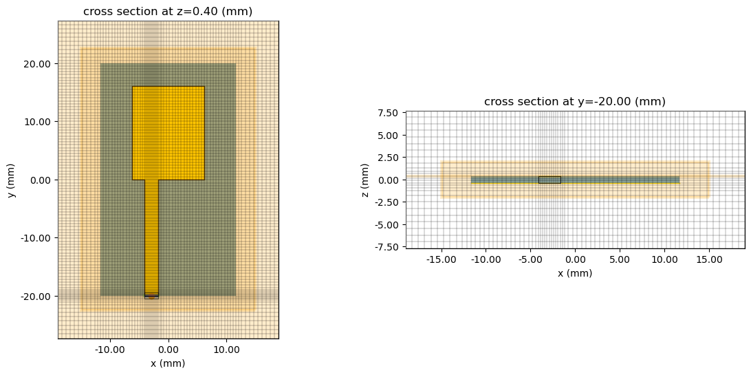
Examine Structures and Mesh
Before running the simulation, it is advisable to inspect the created structure and mesh.
Here, we examine the structure along its propagation direction and the cross-section at the terminated end of the feed line, which includes the location of the lumped port (green with red arrow).
# Create plot
fig, (ax1, ax2) = plt.subplots(1, 2, figsize=(12, 6))

# Plot the structure and mesh in the x-y plane
modeler.plot_sim(
    z=sub_z / 2,
    ax=ax1,
    monitor_alpha=0.2,
)
sim.plot_grid(z=sub_z / 2, ax=ax1, hlim=[-20 * mm, 20 * mm], vlim=[-25 * mm, 25 * mm])

# Plot the structure and mesh in the x-z plane
modeler.plot_sim(
    y=-sub_y / 2,
    ax=ax2,
    monitor_alpha=0.2,
)
sim.plot_grid(y=-sub_y / 2, ax=ax2, hlim=[-15 * mm, 15 * mm], vlim=[-1 * mm, 5 * mm])
ax2.set_aspect(5)

plt.show()
Run simulation
Use the tidy3d.web.upload() method to upload the job and get a cost estimate.
task_id = web.upload(modeler, task_name="antenna_modeler")
             WARNING:  ℹ️ ⚠️ RF simulations are subject to new license
             requirements in the future. You are using RF-specific components in
             this simulation.
              - Contains a 'LumpedElement'.
              - Contains monitors defined for RF wavelengths.
             WARNING: Structure: simulation.structures[4] (no `name` was
             specified) has geometry with zero size along dimensions [1], and
             with a medium that is not a 'Medium2D'. This is probably not
             correct, since the resulting simulation will depend on the details
             of the numerical grid. Consider either giving the geometry a
             nonzero thickness or using a 'Medium2D'.
11:00:22 EST Created task 'antenna_modeler' with resource_id
             'sid-5a46b5d7-3e7f-46f6-bbc9-d35632b9e4f2' and task_type
             'TERMINAL_CM'.
             View task using web UI at
             'https://tidy3d.simulation.cloud/rf?taskId=pa-cddf633f-4745-403f-91
             1a-a42742a2df8b'.
Task folder: 'default'.
Output()
11:00:31 EST Maximum FlexCredit cost: 0.097. Minimum cost depends on task
             execution details. Use 'web.real_cost(task_id)' after run.
We start and monitor the job below.
# Run and monitor simulation
web.start(task_id)
web.monitor(task_id)
11:00:32 EST Subtasks status - antenna_modeler
             Group ID: 'pa-cddf633f-4745-403f-911a-a42742a2df8b'
Output()
Batch status = preprocess
11:00:39 EST Batch status = running
11:01:24 EST Batch status = postprocess
11:01:47 EST Modeler has finished running successfully.
11:01:48 EST Billed flex credit cost: 0.082.
After completion, we download the TCM data.
# Load TCM data
tcm_data = web.load(task_id)
Output()
11:01:53 EST Loading component modeler data from cm_data.hdf5
             WARNING:  ℹ️ ⚠️ RF simulations are subject to new license
             requirements in the future. You are using RF-specific components in
             this simulation.
              - Contains a 'LumpedElement'.
              - Contains sources defined for RF wavelengths.
              - Contains monitors defined for RF wavelengths.
We can also check the real cost of the simulation.
# Print real sim cost
_ = web.real_cost(task_id)
11:01:54 EST Billed flex credit cost: 0.082.
Use the smatrix() method of the TCM data object to calculate the S-matrix.
s_matrix = tcm_data.smatrix()
Results
S-parameters
The s_matrix returned by the TerminalComponentModeler is the full fxNxN matrix, where f is the number of frequency points and N is the number of ports. In this case, there is only one port.
Note that Tidy3D uses the physics phase convention. We apply complex conjugate to the calculated S-parameter in order to convert it to the engineering convention. The latter convention is more commonly used in RF and microwave applications.
# Specify port_in and port_out to get the specific S_ij
S11 = np.conjugate(s_matrix.data.isel(port_out=0, port_in=0))

# Transform to dB
S11dB = 20 * np.log10(np.abs(S11))
# Plot S11dB
fig, ax = plt.subplots()
ax.plot(
    freqs / 1e9,
    S11dB,
    "-b",
)
ax.set_xlabel("Frequency (GHz)")
ax.set_ylabel("$|S_{11}|^2$ (dB)")
ax.grid(True)
plt.show()
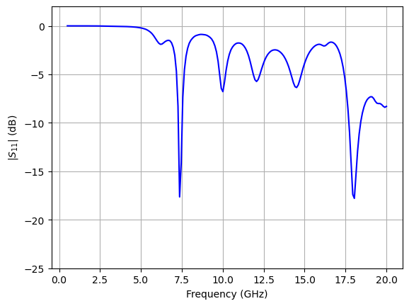
The first and second resonances are clearly visible in the S11 spectrum. Let's examine the field profile next.
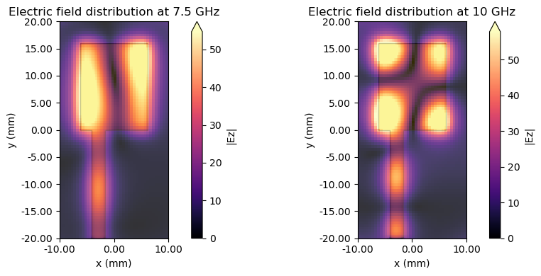
Field Distributions
The dictionary stored in the data attribute of the TerminalComponentModelerData instance contains all the monitor data. Use the respective port name as the dictionary key to access the data associated with the desired port excitation.
# Get simulation data associated with the lumped port excitation
sim_data = tcm_data.data["lumped_port"]
Below, we plot the fields at the first two resonances.
# Plot field monitor data
f, (ax1, ax2) = plt.subplots(1, 2, figsize=(11, 4))
sim_data.plot_field(
    field_monitor_name="field", field_name="Ez", val="abs", f=freqs_target[0], ax=ax1
)
ax1.set_xlim([-10 * mm, 10 * mm])
ax1.set_ylim([-20 * mm, 20 * mm])
ax1.set_title("Electric field distribution at 7.5 GHz")

sim_data.plot_field(
    field_monitor_name="field", field_name="Ez", val="abs", f=freqs_target[1], ax=ax2
)
ax2.set_xlim([-10 * mm, 10 * mm])
ax2.set_ylim([-20 * mm, 20 * mm])
ax2.set_title("Electric field distribution at 10 GHz")
plt.show()
Impedance
The antenna impedance can be calculated from S11.
First, we need to de-embed S11 to account for the length of the feed line. The de-embedding calculation shifts the S11 reference plane from the location of the lumped port ($y = -20$ mm) to the end of the feed line where it connects to the patch ($y = 0$ mm).
In general terms, the de-embedded S-parameter $$ S_\text{de-embedded} = S\exp(2jkL) $$ where $S$ is the original S-parameter, $k$ is the waveguide wavenumber, and $L$ is the shift distance. For simplicity, we assume that the microstrip feed line has a constant effective permittivity of $1.9$ and characteristic impedance of $Z_0=50$ Ohms.
# Wavenumber associated with microstrip feed line
k_microstrip = 2 * np.pi * freqs * np.sqrt(1.9) / td.C_0

# De-embedded S-parameter
S11_deembedded = S11 * np.exp(1j * 2 * k_microstrip * feed_y)
The antenna impedance can then be calculated using the de-embedded S11.
$$ Z_\text{ant} = Z_0 \frac{1+S11_\text{de-embedded}}{1-S11_\text{de-embedded}} $$
# Antenna impedance
Z_ant = 50 * (1 + S11_deembedded) / (1 - S11_deembedded)
Let's plot the antenna impedance near the first resonance. We observe a very good match with $Z_0$ at resonance.
# Plot antenna impedance near first resonance f=7.5 Ghz
fig, ax = plt.subplots()
ax.plot(freqs / 1e9, np.real(Z_ant), label="Re Z")
ax.plot(freqs / 1e9, np.imag(Z_ant), label="Im Z")
ax.axline((7.5, -50), (7.5, 50), ls="--", color="#555555", label="f=7.5 GHz")
ax.set_xlim(7, 8)
ax.set_ylim(-40, 60)
ax.legend()
ax.set_xlabel("f (GHz)")
ax.set_ylabel("Impedance (Ohms)")
ax.grid()
plt.show()
Far-field Metrics
Directivity, gain and other commonly used antenna metrics are automatically calculated when one or more radiation_monitor is defined. The user can obtain the far-field metrics by calling the get_antenna_metrics_data() method on the TCM data object.
# Get antenna metrics
antenna_metrics = tcm_data.get_antenna_metrics_data()
Below, we list all of the available antenna far-field metrics for the user's reference.
# The available antenna metrics quantities are listed below:
# Directivity
directivity = antenna_metrics.directivity
# Radiation efficiency: efficiency accounting for material losses
radiation_efficiency = antenna_metrics.radiation_efficiency
# Gain: radiation efficiency * directivity
gain = antenna_metrics.gain
# Reflection efficiency: efficiency accounting for impedance mismatch
reflection_efficiency = antenna_metrics.reflection_efficiency
# Realized gain: reflection efficiency * gain
realized_gain = antenna_metrics.realized_gain
# Supplied power: power supplied to antenna
supplied_power = antenna_metrics.supplied_power
# Radiated power: power radiated by antenna
radiated_power = antenna_metrics.radiated_power
# Radiation intensity: radiated intensity as a function of angle
radiation_intensity = antenna_metrics.radiation_intensity
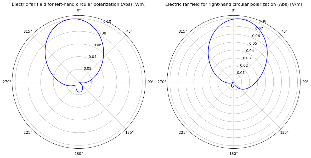
# Axial ratio: ratio of major axis to minor axis of polarization ellipse
axial_ratio = antenna_metrics.axial_ratio
# Left and right circular polarization field components
left_polarization = antenna_metrics.left_polarization
right_polarization = antenna_metrics.right_polarization
In the following sections, we will demonstrate how to plot the gain and axial ratio.
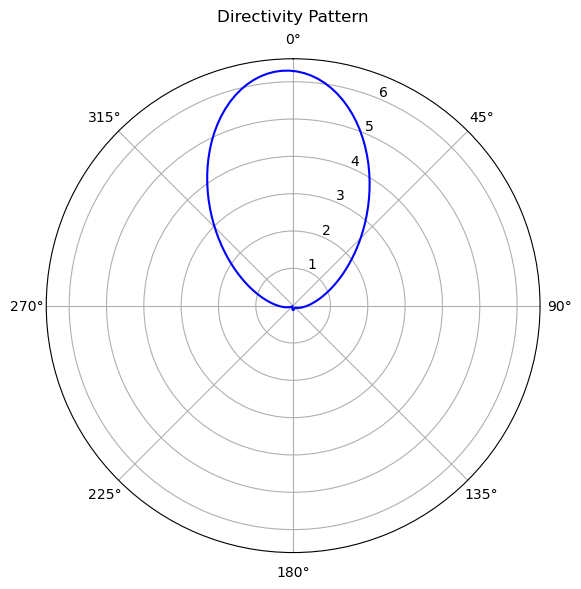
Antenna Gain
Let's plot the gain at the first resonance (f=7.5 GHz).
# Plot gain in elevation plane at f=7.5 GHz

# First, extract gain data in the forward and backward directions
gain_F = gain.sel(f=freqs_target[0], phi=0, method="nearest").squeeze()
gain_B = gain.sel(f=freqs_target[0], phi=-np.pi, method="nearest").squeeze()

# Create plot
fig = plt.figure(figsize=(8, 6), tight_layout=True)
ax = fig.add_subplot(111, projection="polar")

# Plot gain in dB
ax.set_theta_direction(-1)
ax.set_theta_offset(np.pi / 2.0)
ax.plot(theta, 20 * np.log10(np.abs(gain_F)), "-b")
ax.plot(-theta, 20 * np.log10(np.abs(gain_B)), "-b")
ax.set_title("Antenna Gain (dB) in XZ plane")
plt.show()
# Plot gain in azimuthal plane at f=7.5 GHz

# Extract gain in azimuthal plane
gain_azi = gain.sel(f=freqs_target[0], theta=np.pi / 2, method="nearest").squeeze()

# Create plot
fig = plt.figure(figsize=(8, 6), tight_layout=True)
ax = fig.add_subplot(111, projection="polar")

# Plot gain in dB
ax.plot(phi, 20 * np.log10(np.abs(gain_azi)), "-b")
ax.set_title("Antenna Gain (dB) in XY plane")
plt.show()
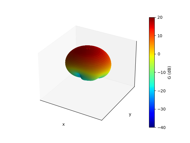
We can also create a 3D plot of the gain.
# Activate interactive plotting (useful for 3D)
# Requires ipympl library to be installed (comment line below if requirement not met)
%matplotlib widget
# Create figure and axes
fig_3d = plt.figure()
ax_3d = fig_3d.add_subplot(1, 1, 1, projection="3d")
limits = 1.0
ax_3d.set_xlim(-limits, limits)
ax_3d.set_ylim(-limits, limits)
ax_3d.set_zlim(-limits, limits)
ax_3d.set_xticks([])
ax_3d.set_yticks([])
ax_3d.set_zticks([])
ax_3d.set_xlabel("x")
ax_3d.set_ylabel("y")
ax_3d.set_zlabel("z")

# Rescale gain according to max and min dB values
dB_min, dB_max = (-40, 20)
G = 20 * np.log10(np.abs(gain.sel(f=7.5e9, method="nearest").squeeze()))
G_scaled = np.clip((G - dB_min) / (dB_max - dB_min), a_min=0, a_max=1)

# Create 3D dataset according to scaled gain
phi_s, theta_s = np.meshgrid(phi, theta)
X = G_scaled * np.cos(phi_s) * np.sin(theta_s)
Y = G_scaled * np.sin(phi_s) * np.sin(theta_s)
Z = G_scaled * np.cos(theta_s)

# Select color map
color_map = plt.cm.jet

# Plot surface
surf = ax_3d.plot_surface(
    X,
    Y,
    Z,
    cstride=2,
    rstride=2,
    facecolors=color_map(G_scaled),
)

# Plot color bar
cbar = fig_3d.colorbar(
    plt.cm.ScalarMappable(norm=colors.Normalize(vmax=dB_max, vmin=dB_min), cmap=color_map),
    ax=ax_3d,
    label="G (dB)",
)
plt.show()
# Close 3D figure and deactivate interactive plotting
plt.close(fig_3d)
%matplotlib inline
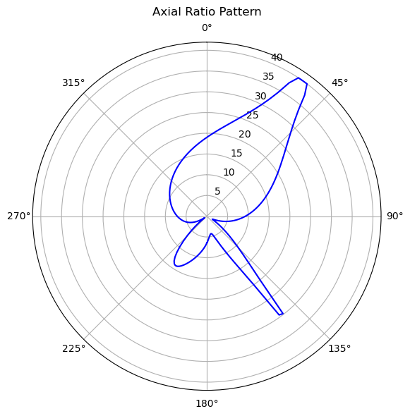
Axial Ratio
Let's plot the axial ratio vs frequency for the main lobe (phi, theta = 0)
# Extract axial ratio at main lobe
axial_ratio_main_lobe = axial_ratio.sel(theta=0, phi=0, method="nearest").squeeze()
# Plot main lobe axial ratio vs frequency
fig, ax = plt.subplots()
ax.plot(freqs / 1e9, 10 * np.log10(axial_ratio_main_lobe))
ax.grid()
ax.set_xlabel("f (GHz)")
ax.set_ylabel("Axial ratio (dB)")
plt.show()
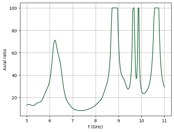
Note that the axial ratio is capped during post-processing at a maximum value of 100, i.e. radiation is effectively linearly polarized.
Reference
[1] Sheen, D.M., Ali, S.M., Abouzahra, M.D. and Kong, J.A., 1990. Application of the three-dimensional finite-difference time-domain method to the analysis of planar microstrip circuits. IEEE Transactions on microwave theory and techniques, 38(7), pp.849-857.

