The demand for ever higher input/output (I/O) bandwidths has driven the development of co-packaged optics (CPO), where optical components are integrated alongside the application-specific integrated circuit (ASIC). This approach enables higher transmission rates and lower energy consumption, helping to circumvent the packaging bottlenecks that limit next-generation communication devices.
A natural evolution is to bring the optics directly onto the silicon interposer, reducing the electrical distance between transmitter/receiver and ASIC. This tighter integration is particularly relevant for datacenters, high-performance computing (HPC) clusters, and AI systems, where switch bandwidth and energy efficiency are critical.
At the same time, chip power continues to rise, requiring increasingly complex cooling solutions. Thermal management becomes a central challenge, since temperature variations directly impact the performance of microring modulators and filters used in dense wavelength-division multiplexing (DWDM) links.
In this notebook, we illustrate how to set up a simplified 3D thermal simulation of a microring integrated on a silicon interposer, inspired by the paper of Benjamin G. Lee, Nikola Nedovic, Thomas H. Greer, and C. Thomas Gray, "Beyond CPO: A Motivation and Approach for Bringing Optics Onto the Silicon Interposer", Journal of Lightwave Technology 41(4), 1152–1165 (2023). DOI: https://doi.org/10.1109/JLT.2022.3219379.
The key steps are:
-
Define the material stack — silicon interposer, buried oxide, photonic layer, BEOL glass, copper heat spreader, and heaters.
-
Assign thermal properties — capacity, conductivity, and density for each material.
-
Set up boundary conditions — insulating boundaries, with thermal impedance applied at the top of the heat spreader.
-
Apply power perturbations — ASIC load steps and local heater power steps.
-
Run transient simulations — compute the time-dependent temperature distribution across the device.
-
Analyze results — observe the thermal response of the microring, neighbor coupling, and evaluate stabilization requirements for control loops.
import matplotlib.pyplot as plt
import numpy as np
import tidy3d as td
import tidy3d.web as web
Simulation Setup
First we will define an auxiliary function to easily stack the different parts of the geometry.
def stack_box(
    structure_1,
    structure_2,
    plane="x",
    horizontal="right",
    vertical="top",
    gap_h=0,
    gap_v=0,
    new_name=None,
):
    """
    Aligns and stacks *structure_2* relative to *structure_1* in a given plane
    with configurable horizontal and vertical positioning.

    Parameters
    ----------
    structure_1 : tidy3d.Structure
        Tidy3D structure used as the base.
    structure_2 : tidy3d.Structure
        Tidy3D structure to be translated and stacked relative to *structure_1*.
    plane : str, optional
        Plane of alignment ('x', 'y', or 'z'). Default is 'x'.
    horizontal : str, optional
        Horizontal alignment relative to *structure_1* ('left', 'right', 'center').
        Default is 'right'.
    vertical : str, optional
        Vertical alignment relative to *structure_1* ('top', 'bottom', 'center').
        Default is 'top'.
    gap_h : float, optional
        Horizontal gap between structures. Default is 0.
    gap_v : float, optional
        Vertical gap between structures. Default is 0.
    new_name : str, optional
        Name for the updated *structure_2*. If None, retains original name.

    Returns
    -------
    tidy3d.Structure
        A copy of *structure_2* translated to the new aligned position.
    """

    box_1 = structure_1.geometry.bounding_box
    box_2 = structure_2.geometry.bounding_box

    c1 = np.array(box_1.center)
    c2 = np.array(box_2.center)

    s1 = np.array(box_1.size)
    s2 = np.array(box_2.size)

    # Default: new center is box_1 center
    new_center = c1.copy()

    # Which plane are we stacking in?
    axis = {"x": 0, "y": 1, "z": 2}[plane]
    aux = [0, 1, 2]
    aux.remove(axis)
    horizontal_axes = min(aux)
    vertical_axes = max(aux)

    for i in [(horizontal, horizontal_axes, gap_h), (vertical, vertical_axes, gap_v)]:
        if i[0] == "center":
            new_center[i[1]] = c1[i[1]]
        elif i[0] == "left":
            new_center[i[1]] = c1[i[1]] - s1[i[1]] / 2 + (s2[i[1]] / 2) + i[2]
        elif i[0] == "right":
            new_center[i[1]] = c1[i[1]] + s1[i[1]] / 2 - (s2[i[1]] / 2) + i[2]
        elif i[0] == "top":
            new_center[i[1]] = c1[i[1]] + s1[i[1]] / 2 + (s2[i[1]] / 2) + i[2]
        elif i[0] == "bottom":
            new_center[i[1]] = c1[i[1]] - s1[i[1]] / 2 - (s2[i[1]] / 2) - i[2]

    translated_geometry = structure_2.geometry.translated(
        x=-c2[0] + new_center[0], y=-c2[1] + new_center[1], z=-c2[2] + new_center[2]
    )

    return structure_2.updated_copy(
        geometry=translated_geometry, name=new_name if new_name else structure_2.name
    )
Material properties
For heating simulations, we need to add a heat specification to the Tidy3D MultiPhysicsMedium object via the heat_spec argument, defining the thermal material properties:
- Specific heat capacity in J/(kg·K)
- Thermal conductivity in W/(µm·K)
- Density in kg/µm³, required for transient heat analysis
Si_n = 3.4777  # Si refractive index
Si_n_slope = 1.86e-4  # Si thermo-optic coefficient dn/dT [1/K]

Si_capacity = 710  # Si specific heat capacity [J/(kg·K)]
Si_conductivity = 148e-6  # Si thermal conductivity [W/(µm·K)]
Si_density = 2.33e-15  # Si density [kg/µm^3] (2330 kg/m^3)

freq0 = td.C_0 / 1.5

Si_optical = td.Medium.from_nk(n=Si_n, k=0, freq=freq0)
Si_heat = td.SolidSpec(capacity=Si_capacity, conductivity=Si_conductivity, density=Si_density)

Si = td.MultiPhysicsMedium(optical=Si_optical, heat=Si_heat, name="Si")

SiO2_n = 1.444  # SiO2 refractive index
SiO2_n_slope = 1e-5  # SiO2 thermo-optic coefficient dn/dT [1/K]

SiO2_capacity = 703  # SiO2 specific heat capacity [J/(kg·K)]
SiO2_conductivity = 1.38e-6  # SiO2 thermal conductivity [W/(µm·K)]
SiO2_density = 2.634e-15  # SiO2 density [kg/µm^3] (2634 kg/m^3)

# Alternative way of defining a medium specification
SiO2_optical = td.Medium(permittivity=SiO2_n**2)

SiO2_heat = td.SolidSpec(
    capacity=SiO2_capacity, conductivity=SiO2_conductivity, density=SiO2_density
)
SiO2 = td.MultiPhysicsMedium(optical=SiO2_optical, heat=SiO2_heat, name="SiO2")

Cu_capacity = 385  # Cu specific heat capacity [J/(kg·K)]
Cu_conductivity = 401e-6  # Cu thermal conductivity [W/(µm·K)]
Cu_density = 8.96e-15  # Cu density [kg/µm^3] (8960 kg/m^3)

Cu_optical = td.PECMedium()
Cu_heat = td.SolidSpec(capacity=Cu_capacity, conductivity=Cu_conductivity, density=Cu_density)

Cu = td.MultiPhysicsMedium(
    optical=Cu_optical,
    heat=Cu_heat,
    name="Cu",
)

# BEOL layer (modeled as porous SiO2 / low-k dielectric)
BEOL_capacity = 703  # J/(kg·K), similar to SiO2
BEOL_conductivity = 0.45e-6  # W/(µm·K), reduced effective conductivity
BEOL_density = 2.2e-15  # kg/µm^3, lower density due to porosity

beol_SiO2_optical = td.Medium(permittivity=SiO2_n**2)
beol_SiO2_heat = td.SolidSpec(
    capacity=BEOL_capacity,
    conductivity=BEOL_conductivity,
    density=BEOL_density,
)

beol_SiO2 = td.MultiPhysicsMedium(
    optical=beol_SiO2_optical,
    heat=beol_SiO2_heat,
    name="BEOL",
)
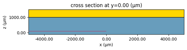
Simulation Geometry
Next, we will define the different layers of the structure.
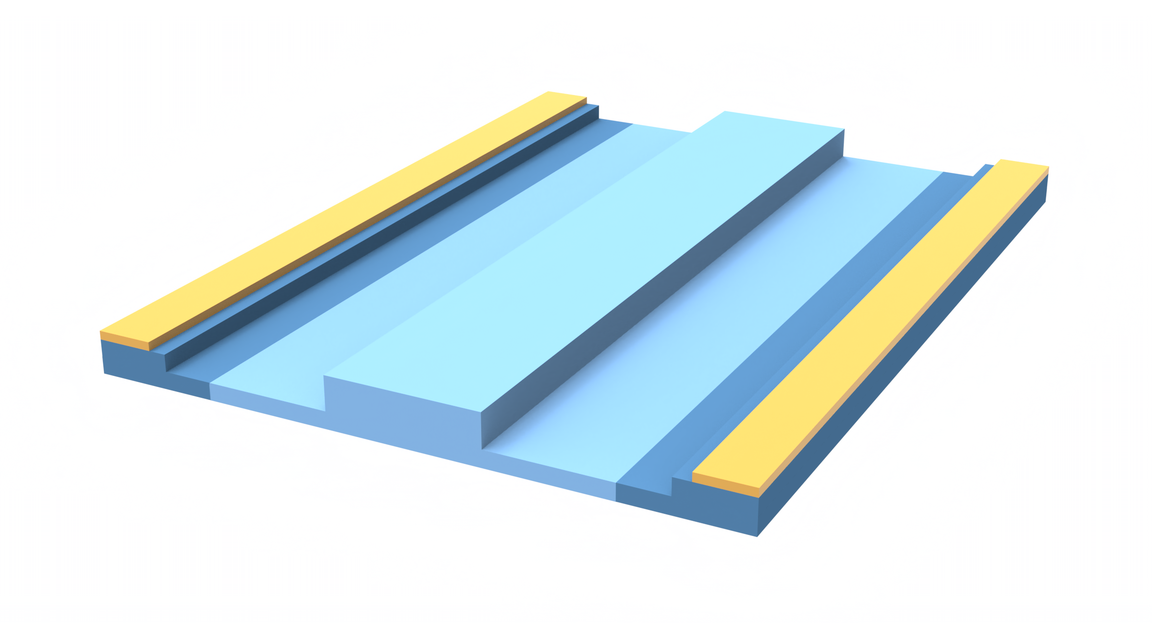
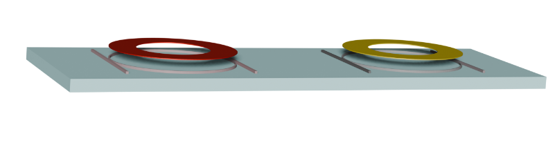
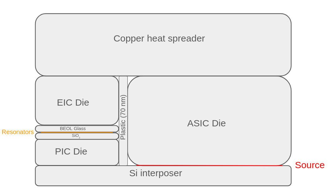
The stack consists of:
- Copper heat spreader on top, which serves as the main cooling interface.
- ASIC (logic die), the primary heat source in the system.
- Plastic molding compound as a thin spacer between the ASIC and the photonic layers.
- Photonic Integrated Circuit (PIC) on the interposer surface, containing the microring resonators.
- Buried oxide (BOX) below the silicon waveguides, providing thermal and optical isolation.
- BEOL glass above the rings, insulating them from the electronic circuits.
- Metal heaters embedded in glass just above the rings for thermo-optic tuning.
- Silicon interposer at the bottom.
A schematic can be seen in the image below:
# Unit helpers (all geometry in µm)
mm = 1e3
width = 160 * mm

# Silicon interposer (bottom substrate, 100 µm thick in the paper)
interposer_thickness = 0.1 * mm
interposer_length = 10 * mm
Silicon_interposer = td.Structure(
    geometry=td.Box(
        center=(0, 0, -interposer_thickness / 2),
        size=(interposer_length, width, interposer_thickness),
    ),
    name="Silicon_interposer",
    medium=Si,
)

# ASIC die (logic die, ~1 mm thick)
asic_thickness = 1 * mm
asic_length = 5 * mm
ASIC_Die = td.Structure(
    geometry=td.Box(size=(asic_length, width, asic_thickness)),
    name="ASIC_Die",
    medium=Si,
)

# Plastic molding compound spacer between ASIC and PIC/EIC (~70 nm)
silicon_gap_thickness = 0.07  # 70 nm
silicon_gap_length = 10 * mm
Silicon_gap = td.Structure(
    geometry=td.Box(size=(silicon_gap_length, width, silicon_gap_thickness)),
    name="Molding_spacer",
    medium=SiO2,  # simple proxy; replace with a polymer if desired
)

# Optional placeholder “source region” (e.g., for heater or power injection)
Source = td.Structure(
    geometry=td.Box(size=(5 * mm, width, 0.01)),  # 10 nm
    name="Source",
    medium=Si,  # set to appropriate medium if used
)

# PIC die on interposer (photonic Si layer stack)
buried_sio2_thickness = 2  # µm (BOX)
beol_thickness = 10  # µm (BEOL glass)

# Photonic Si core (100 µm total PIC die; subtract BOX and BEOL to keep total)
pic_thickness = 0.1 * mm
pic_length = 5 * mm
PIC_Die = td.Structure(
    geometry=td.Box(
        size=(pic_length, width, pic_thickness - buried_sio2_thickness - beol_thickness)
    ),
    name="PIC_Die",
    medium=Si,
)

# Buried oxide (BOX) under the photonic Si
buried_sio2 = td.Structure(
    geometry=td.Box(size=(pic_length, width, buried_sio2_thickness)),
    name="buried_sio2",
    medium=SiO2,
)

# BEOL dielectric above the photonic Si (glass/low-k stack)
beol = td.Structure(
    geometry=td.Box(size=(pic_length, width, beol_thickness)),
    name="beol",
    medium=beol_SiO2,
)

# EIC die above the PIC (fills remaining thickness up to ~1 mm total)
eic_thickness = 1 * mm - pic_thickness
eic_length = pic_length
EIC_Die = td.Structure(
    geometry=td.Box(size=(eic_length, width, eic_thickness)),
    name="EIC_Die",
    medium=Si,
)

# Copper heat spreader on top (~0.5 mm)
heat_spreader_thickness = 0.5 * mm
heat_spreader_length = 10 * mm
Heat_spreader = td.Structure(
    geometry=td.Box(size=(heat_spreader_length, width, heat_spreader_thickness)),
    name="Heat_spreader",
    medium=Cu,
)


# Lateral gap placeholder
die_gap_thickness = asic_thickness
die_gap_length = 0.07  # 70 nm in x
Die_gap = td.Structure(
    geometry=td.Box(size=(die_gap_length, width, die_gap_thickness)),
    name="Die_gap_lateral",
    medium=SiO2,
)

# Stack the structures (using your helper `stack_box`)
ASIC_Die = stack_box(Silicon_interposer, ASIC_Die, plane="y", horizontal="right", vertical="top")
PIC_Die = stack_box(Silicon_interposer, PIC_Die, plane="y", horizontal="left", vertical="top")
buried_sio2 = stack_box(PIC_Die, buried_sio2, plane="y", horizontal="left", vertical="top")
beol = stack_box(buried_sio2, beol, plane="y", horizontal="left", vertical="top")
EIC_Die = stack_box(beol, EIC_Die, plane="y", horizontal="center", vertical="top")
Die_gap = stack_box(ASIC_Die, Die_gap, plane="y", horizontal="left", vertical="center")
Heat_spreader = stack_box(EIC_Die, Heat_spreader, plane="y", horizontal="left", vertical="top")
scene = td.Scene(
    structures=[
        Silicon_interposer,
        #  Silicon_gap,
        ASIC_Die,
        PIC_Die,
        EIC_Die,
        Die_gap,
        Heat_spreader,
        beol,
        buried_sio2,
    ]
)

ax = scene.plot(y=0)

plt.show()
Defining Mesh
We will use a DistanceUnstructuredGrid object to create a mesh that is finer around interfaces.
dl = 0.005 * mm
mesh = td.UniformUnstructuredGrid(dl=dl, relative_min_dl=0.0003)
Defining Source
Here, we will use a linear source at the bottom of the ASIC die. The HeatSource object is assigned to the ASIC die structure, with a custom power distribution only at its bottom.
# Line heat source

x = np.linspace(0 * mm, 5 * mm, 100)
y = [0]
z = [0]

rate = 2 * (500 / 800) * 1e-9  # W/um^3
data = rate * np.ones((len(x), 1, 1))


coords = dict(x=x, y=y, z=z)
custom_rate = td.SpatialDataArray(data, coords=coords)

heat_source = td.HeatSource(structures=["ASIC_Die"], rate=custom_rate)  # W/um^3
Defining Monitors
We will add a TemperatureMonitor to track the temperature distribution across the simulation domain.
temp_mnt = td.TemperatureMonitor(size=(td.inf, 0, td.inf), name="temperature", unstructured=True)
Boundary Conditions
The boundary conditions are all insulating, except for the z+ boundary, which uses a ConvectionBC with a heat impedance of $3\times10^7 \mu\text{m}^2\text{ K/W}$.
insulating = td.HeatBoundarySpec(
    condition=td.HeatFluxBC(flux=0),
    placement=td.SimulationBoundary(surfaces=["x+", "x-", "z-"]),
)

heat_impedance = 3e7  # µm^2 K/W

top_boundary = td.HeatBoundarySpec(
    condition=td.ConvectionBC(
        ambient_temperature=300,  # K
        transfer_coeff=1 / heat_impedance,  # W/(K*µm^2)
    ),
    placement=td.SimulationBoundary(surfaces=["z+"]),
)
Steady Heat Simulation
First, we will assemble all components and create the HeatChargeSimulation object for the steady-state simulation.
We can see warnings regarding structures extending into the PML
# Set the simulation size to be slightly smaller than the scene size to avoid warnings
# Set the size in y to 0 (structures are translationally invariant in y)
size = [s * 0.99 for s in scene.size]
size[1] = dl
heat_sim = td.HeatChargeSimulation(
    center=scene.center,
    size=size,
    medium=scene.medium,
    structures=scene.structures,
    boundary_spec=[insulating, top_boundary],
    sources=[heat_source],
    grid_spec=mesh,
    monitors=[temp_mnt],
)
Finally, we can use web.run to upload the simulation to the cloud, run it, monitor progress, download the data, and load it into the HeatChargeSimulationData object for post-processing.
steady_data = web.run(heat_sim, task_name="CPOHeat_Steady")
11:54:27 CET Created task 'CPOHeat_Steady' with resource_id
             'hec-6235821f-c122-4d4e-a669-011a5e3a3bbe' and task_type
             'HEAT_CHARGE'.
             Tidy3D's HeatCharge solver is currently in the beta stage. Cost of
             HeatCharge simulations is subject to change in the future.
Output()
11:54:31 CET Estimated FlexCredit cost: 0.025. Minimum cost depends on task
             execution details. Use 'web.real_cost(task_id)' to get the billed
             FlexCredit cost after a simulation run.
11:54:33 CET status = success
Output()
11:54:48 CET Loading results from simulation_data.hdf5
11:54:57 CET WARNING: Warning messages were found in the solver log. For more
             information, check 'SimulationData.log' or use
             'web.download_log(task_id)'.
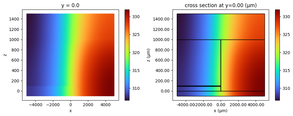
Visualizing Steady-State Results
We can call the .plot method to visualize the field distribution in the simulation plane.
As we can see, the thin plastic region provides good insulation for the ASIC die. For reference, the structures are highlighted in the figure on the right.
fig, (ax, ax2) = plt.subplots(1, 2, figsize=(10, 4))


steady_data["temperature"].temperature.plot(grid=False, ax=ax)
ax.set_aspect("auto")
ax.collections[-1].set_cmap("turbo")

steady_data["temperature"].temperature.plot(grid=False, ax=ax2)
scene.plot(y=0, ax=ax2, fill_structures=False)
ax2.set_aspect("auto")
ax2.collections[-1].set_cmap("turbo")

ax2.set_xlim(ax.get_xlim())
ax2.set_ylim(ax.get_ylim())

plt.tight_layout()
plt.show()
Transient Analysis
For transient heating analysis, the only modification is providing an UnsteadyHeatAnalysis object to the analysis_spec parameter of the HeatChargeSimulation model object, specifying the initial temperature, number of time steps, and step size.
We will reuse the previously created object and update it with the updated_copy method.
time_step_2d = 1e-2
total_time_steps_2d = 100

time_spec = td.UnsteadyHeatAnalysis(
    initial_temperature=300,
    unsteady_spec=td.UnsteadySpec(
        time_step=time_step_2d,
        total_time_steps=total_time_steps_2d,
    ),
)

heat_sim_transient = heat_sim.updated_copy(analysis_spec=time_spec)
12:24:42 CET WARNING: The simulation time is larger than 100 times the estimated
             characteristic time of the system. This may lead to unnecessary
             long simulation times. Consider reducing the simulation time or the
             time step size.
heat_data_transient = web.run(heat_sim_transient, "CPO_2D_Transient")
12:24:43 CET WARNING: The simulation time is larger than 100 times the estimated
             characteristic time of the system. This may lead to unnecessary
             long simulation times. Consider reducing the simulation time or the
             time step size.
12:24:44 CET Created task 'CPO_2D_Transient' with resource_id
             'hec-ebfe580c-522f-4151-8125-60115dee6489' and task_type
             'HEAT_CHARGE'.
             Tidy3D's HeatCharge solver is currently in the beta stage. Cost of
             HeatCharge simulations is subject to change in the future.
Output()
12:24:48 CET Estimated FlexCredit cost: 0.025. Minimum cost depends on task
             execution details. Use 'web.real_cost(task_id)' to get the billed
             FlexCredit cost after a simulation run.
12:24:51 CET status = success
Output()
12:27:34 CET Loading results from simulation_data.hdf5
12:27:52 CET WARNING: The simulation time is larger than 100 times the estimated
             characteristic time of the system. This may lead to unnecessary
             long simulation times. Consider reducing the simulation time or the
             time step size.
12:27:55 CET WARNING: Warning messages were found in the solver log. For more
             information, check 'SimulationData.log' or use
             'web.download_log(task_id)'.
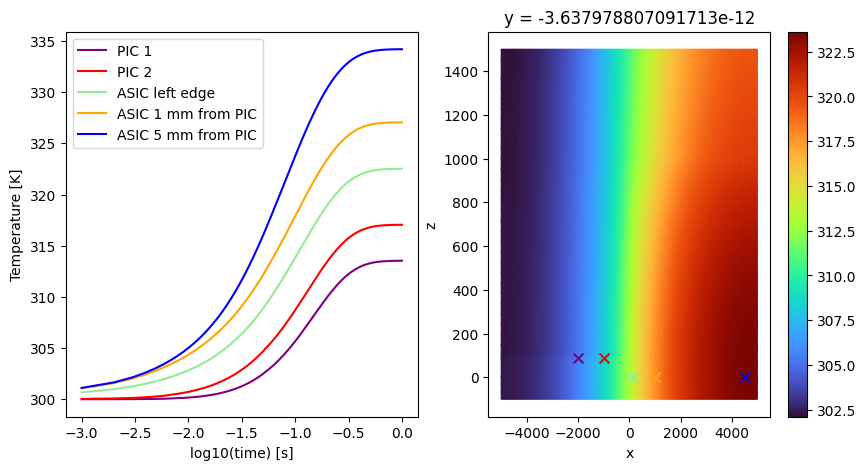
Visualizing Transient Results
Next we will visualize the results at typical resonator positions and at different points on the ASIC die.
fig, Ax = plt.subplots(1, 2, figsize=(10, 5))

PIC_z = buried_sio2.geometry.bounding_box.center[2]

temp1 = heat_data_transient["temperature"].temperature.sel(x=-2000, z=PIC_z, method="nearest")
temp2 = heat_data_transient["temperature"].temperature.sel(x=-1000, z=PIC_z, method="nearest")
temp3 = heat_data_transient["temperature"].temperature.sel(x=100, z=0, method="nearest")
temp4 = heat_data_transient["temperature"].temperature.sel(x=1000, z=0, method="nearest")
temp5 = heat_data_transient["temperature"].temperature.sel(x=4500, z=0, method="nearest")


time_steps = time_step_2d * np.arange(1, total_time_steps_2d + 1)

Ax[0].plot(np.log10(time_steps), temp1.values.squeeze(), color="purple", label="PIC 1")
Ax[0].plot(np.log10(time_steps), temp2.values.squeeze(), color="red", label="PIC 2")
Ax[0].plot(np.log10(time_steps), temp3.values.squeeze(), color="lightgreen", label="ASIC left edge")
Ax[0].plot(np.log10(time_steps), temp4.values.squeeze(), color="orange", label="ASIC 1 mm from PIC")
Ax[0].plot(np.log10(time_steps), temp5.values.squeeze(), color="blue", label="ASIC 5 mm from PIC")
Ax[0].set_xlabel("log10(time) [s]")
Ax[0].set_ylabel("Temperature [K]")
Ax[0].legend()

_ = heat_data_transient["temperature"].temperature.isel(t=99).plot(grid=False, ax=Ax[1])
Ax[1].set_aspect("auto")
Ax[1].collections[-1].set_cmap("turbo")
Ax[1].scatter(-2000, PIC_z, color="purple", s=50, marker="x")
Ax[1].scatter(-1000, PIC_z, color="red", s=50, marker="x")
Ax[1].scatter(100, 0, color="lightgreen", s=50, marker="x")
Ax[1].scatter(1000, 0, color="orange", s=50, marker="x")
Ax[1].scatter(4500, 0, color="blue", s=50, marker="x")

plt.show()
3D Transient Simulation
Now we will investigate the effect of the heater on neighboring resonators.
A localized power step is applied to one microring heater, and the transient temperature response is computed in 3D.
This allows us to observe the ring’s heating dynamics and quantify thermal crosstalk with adjacent resonators.
Defining the Ring and Heater Geometry
# Ring center (aligned above the buried oxide layer)
mrr_center = (
    -2000,
    0,
    buried_sio2.geometry.bounding_box.center[2] + buried_sio2.geometry.bounding_box.size[2] / 2,
)

# Heater placed 1 µm above the ring center in z
heater_center = (mrr_center[0], mrr_center[1], mrr_center[2] + 1)

# Ring dimensions (radius = 20 µm, width = 1 µm)
ring_radius = 20
ring_width = 1

# Ring geometry defined as a hollow cylinder (outer – inner cylinder)
ring_geometry = td.Cylinder(
    center=heater_center, radius=ring_radius, length=0.22, axis=2
) - td.Cylinder(center=heater_center, radius=ring_radius - ring_width, length=0.22, axis=2)

# Define first microring (Si core)
ring1 = td.Structure(geometry=ring_geometry, medium=Si, name="ring")

# Define heater overlapping the ring geometry (Cu)
heater1 = td.Structure(geometry=ring_geometry, medium=Cu, name="heater")

# Place heater above ring1 with a vertical gap of 1 µm
heater1 = stack_box(
    ring1, heater1, plane="y", horizontal="center", vertical="top", gap_v=1, new_name="heater1"
)

# Duplicate ring1 to create a neighboring ring at 100 µm horizontal separation
ring2 = stack_box(
    ring1, ring1, plane="y", horizontal="left", vertical="center", gap_h=100, new_name="ring2"
)

# Place heater above the second ring with the same 1 µm gap
heater2 = stack_box(
    ring2, heater1, plane="y", horizontal="center", vertical="top", gap_v=1, new_name="heater2"
)
The new source is a uniform source located right next to the resonator's heater.
# Line heat source

x = np.linspace(0 * mm, 5 * mm, 100)
y = [0]
z = [0]

power = 5e-3  # 1 mW
volume = 0.22 * np.pi * (ring_radius**2 - (ring_radius - ring_width) ** 2)  # um^3
rate = power / volume  # W/um^3

heat_source3 = td.HeatSource(structures=["heater1"], rate=rate)  # W/um^3
Now we can place the geometry and new source together and update the 2D simulation.
scene_3d = scene.updated_copy(structures=list(scene.structures) + [ring1, heater1, ring2, heater2])

center_3d = mrr_center
size_3d = (1 * mm,) * 3

heat_sim_3d = heat_sim.updated_copy(
    center=center_3d, size=size_3d, structures=scene_3d.structures, sources=[heat_source3]
)
13:43:06 CET WARNING: 'ASIC_Die' (simulation.structures[1]) is outside of the
             simulation domain.
WARNING: Suppressed 2 WARNING messages.
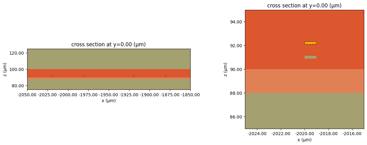
First, let's visualize the geometry:
fig, Ax = plt.subplots(1, 2, figsize=(15, 5))
ax1 = heat_sim_3d.plot(y=0, ax=Ax[0])
ax1.set_xlim(-2050, -1850)
ax1.set_ylim(75, 125)

ax2 = heat_sim_3d.plot(y=0, ax=Ax[1])
ax2.set_xlim(-2025, -2015)
ax2.set_ylim(85, 95)
# ax2.set_aspect('auto')}

plt.show()
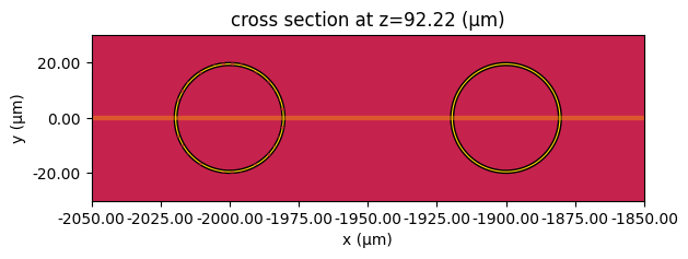
fig, ax = plt.subplots(figsize=(10, 5))
ax = heat_sim_3d.plot(z=heater2.geometry.bounding_box.center[2], ax=ax)
ax.set_xlim(-2050, -1850)
ax.set_ylim(-30, 30)

plt.show()
3D Transient Analysis
Next, we will create an UnsteadyHeatAnalysis object for the 3D analysis and run the simulation.
time_step = 1e-5
total_time_steps = 100

time_spec = td.UnsteadyHeatAnalysis(
    initial_temperature=300,
    unsteady_spec=td.UnsteadySpec(
        time_step=time_step,
        total_time_steps=total_time_steps,
    ),
)

heat_sim_transient_3d = heat_sim_3d.updated_copy(analysis_spec=time_spec)
13:43:13 CET WARNING: 'ASIC_Die' (simulation.structures[1]) is outside of the
             simulation domain.
WARNING: Suppressed 2 WARNING messages.
             WARNING: The simulation time is larger than 100 times the estimated
             characteristic time of the system. This may lead to unnecessary
             long simulation times. Consider reducing the simulation time or the
             time step size.
heat_data_transient_3d = web.run(heat_sim_transient_3d, "CPO_3D_Transient")
15:38:15 CET WARNING: 'ASIC_Die' (simulation.structures[1]) is outside of the
             simulation domain.
WARNING: Suppressed 2 WARNING messages.
             WARNING: The simulation time is larger than 100 times the estimated
             characteristic time of the system. This may lead to unnecessary
             long simulation times. Consider reducing the simulation time or the
             time step size.
15:38:16 CET Created task 'CPO_3D_Transient' with resource_id
             'hec-009cfd59-06a4-439d-80cc-0527ab528521' and task_type
             'HEAT_CHARGE'.
             Tidy3D's HeatCharge solver is currently in the beta stage. Cost of
             HeatCharge simulations is subject to change in the future.
Output()
15:38:20 CET Estimated FlexCredit cost: 0.025. Minimum cost depends on task
             execution details. Use 'web.real_cost(task_id)' to get the billed
             FlexCredit cost after a simulation run.
15:38:22 CET status = success
Output()
15:38:27 CET Loading results from simulation_data.hdf5
             WARNING: 'ASIC_Die' (simulation.structures[1]) is outside of the
             simulation domain.
WARNING: Suppressed 2 WARNING messages.
             WARNING: The simulation time is larger than 100 times the estimated
             characteristic time of the system. This may lead to unnecessary
             long simulation times. Consider reducing the simulation time or the
             time step size.
             WARNING: Warning messages were found in the solver log. For more
             information, check 'SimulationData.log' or use
             'web.download_log(task_id)'.
Visualizing Temperature Distribution
We can now visualize the heat distribution in the heated and neighboring resonators. The crosstalk is very small and can only be seen when saturating the temperature values in the figure on the right.
fig, Ax = plt.subplots(1, 2, figsize=(15, 5))

ax1 = heat_data_transient_3d["temperature"].temperature.isel(t=99).plot(grid=False, ax=Ax[0])
ax1.set_xlim(-2050, -1950)
ax1.set_ylim(75, 125)
ax1.set_title("Heat at the heated resonator")
ax2 = (
    heat_data_transient_3d["temperature"]
    .temperature.isel(t=99)
    .plot(grid=False, ax=Ax[1], vmax=300.1)
)
ax2.set_xlim(-1950, -1850)
ax2.set_ylim(75, 125)
ax2.set_title("Heat at the neighboring resonator")

plt.show()
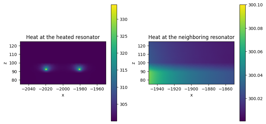
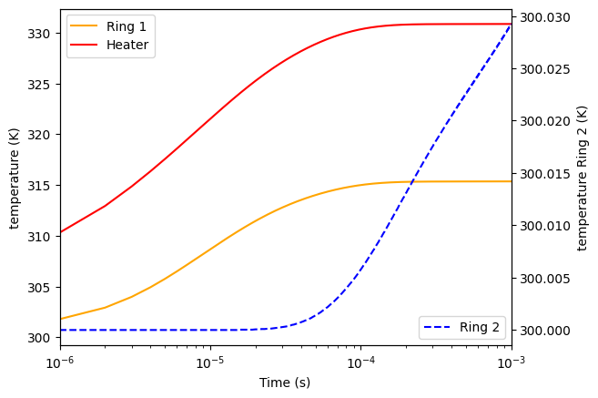
Finally, we can analyze the heat dynamics. As we can see, the heated resonator transient response follows closely the heater, while the neighboring resonator shows only a small temperature rise with a noticeable delay.
This analysis is important for understanding thermal crosstalk between adjacent devices and for defining the requirements for stabilization and control loops that keep the microrings properly tuned.
# Coordinates for sampling temperatures
x_ring_1 = ring1.geometry.bounding_box.center[0] + 19  # sample point near ring radius
y_ring_1 = ring1.geometry.bounding_box.center[1]  # same y as ring center
z_ring_1 = ring1.geometry.bounding_box.center[2]  # same z as ring center

# Temperature at Ring 1
temp_ring1 = heat_data_transient_3d["temperature"].temperature.sel(
    x=x_ring_1,
    z=z_ring_1,
)

# Temperature at Ring 2 (100 µm away in x)
temp_ring2 = heat_data_transient_3d["temperature"].temperature.sel(
    x=x_ring_1 + 100, z=z_ring_1, method="nearest"
)

# Temperature at Heater (1 µm above Ring 1)
temp_heater1 = heat_data_transient_3d["temperature"].temperature.sel(
    x=x_ring_1, z=z_ring_1 + 1, method="nearest"
)

# Plot transients
fig, ax = plt.subplots()

time = time_step * np.arange(total_time_steps)

# Plot Ring 1 and Heater on the primary y-axis
ax.plot(time, temp_ring1.squeeze(), "-", label="Ring 1", color="orange")
ax.plot(time, temp_heater1.squeeze(), "-", label="Heater", color="red")
ax.set_ylabel("temperature (K)")
ax.set_xlabel("Time (s)")
ax.set_xscale("log")
ax.set_xlim(1e-5, 1e-3)
ax.legend(loc=2)

# Plot Ring 2 on a secondary y-axis for clarity
ax2 = ax.twinx()
ax2.plot(time, temp_ring2.squeeze(), "--", label="Ring 2", color="blue")
ax2.set_ylabel("temperature Ring 2 (K)")
ax2.legend(loc=4)


plt.show()