The patch antenna is a ubiquitous antenna type used in modern wireless communication systems. In this notebook, we demonstrate how to simulate a patch antenna using Flexcompute's RF solver and benchmark its performance against a commercial FEM-based full-wave solver. We compare key metrics, such as return loss and gain profile.
import matplotlib.colors as colors
import matplotlib.pyplot as plt
import numpy as np
import tidy3d as td
import tidy3d.rf as rf
import tidy3d.web as web
import xarray as xr
from tidy3d.plugins.dispersion import FastDispersionFitter

td.config.logging.level = "ERROR"
Setup
General Parameters
We will conduct a broadband sweep from 10 MHz to 40 GHz to scan for the resonance(s) of this patch antenna. The target operating frequency of the antenna is around 35.3 GHz.
# Frequency range
f_min, f_max = (0.01e9, 40e9)

# Target operating frequency
f_target = 35.3e9

# Frequency sample points (including f_target)
freqs = np.sort(np.append(np.linspace(f_min, f_max, 301), f_target))
Material and Structures
Both the substrate and conductor materials are assumed to be lossy and have constant loss parameters over the frequency range.
# Lossy substrate (rel. epsilon = 2.2, loss tangent = 0.0009)
med_sub = FastDispersionFitter.constant_loss_tangent_model(
    2.2, 0.0009, (f_min, f_max), tolerance_rms=2e-4
)

# Lossy metal (conductivity = 58e6 S/m)
med_metal = rf.LossyMetalMedium(conductivity=58, frequency_range=(f_min, f_max))
The geometry is constructed below. Note that the default length unit is microns. We introduce a scaling factor mm for convenience.
# Geometry parameters
mm = 1000
t = 0.02 * mm  # Metal thickness
h = 0.254 * mm  # Substrate thickness
# Create substrate and ground planes
str_sub = td.Structure(
    geometry=td.Box(center=(0, 0, -h / 2), size=(6 * mm, 10 * mm, h)), medium=med_sub
)
str_gnd = td.Structure(
    geometry=td.Box(center=(0, 0, -h - t / 2), size=(6 * mm, 10 * mm, t)), medium=med_metal
)

# Create feed structure
str_feed1 = td.Structure(
    geometry=td.Box.from_bounds(rmin=(2 * mm, -0.31 * mm, 0), rmax=(3 * mm, 0.31 * mm, t)),
    medium=med_metal,
)
str_feed2 = td.Structure(
    geometry=td.Box.from_bounds(rmin=(0.5 * mm, -0.05 * mm, 0), rmax=(2 * mm, 0.05 * mm, t)),
    medium=med_metal,
)

# Create antenna structure
ant_vertices = (
    np.array(
        [
            [-1.3, -2.1],
            [-0.3, -2.1],
            [-0.3, -1.1],
            [0.5, -1.1],
            [0.5, 0.6],
            [-0.19, 0.6],
            [-0.19, -0.62],
            [-1.4, -0.62],
            [-1.4, 0.6],
            [-2.1, 0.6],
            [-2.1, -1.1],
            [-1.3, -1.1],
        ]
    )
    * mm
)
str_ant = td.Structure(
    geometry=td.PolySlab(axis=2, slab_bounds=[0, t], vertices=ant_vertices), medium=med_metal
)

# Full structure list
str_list_full = [str_sub, str_gnd, str_feed1, str_feed2, str_ant]
Grid and Boundary
We apply the perfectly matched layer (PML) on all external boundaries. As is standard practice for radiation problems, we also include an air buffer region around the antenna. Typically, the thickness of this padding is wavelength/2 on each side. This is so that the PML does not intrude on and distort the near-field.
# Define simulation size with lambda/2 padding
padding = td.C_0 / f_target / 2
sim_LX = 6 * mm + 2 * padding
sim_LY = 10 * mm + 2 * padding
sim_LZ = 2 * t + h + 2 * padding
# Define PML boundary on all sides
bspec = td.BoundarySpec.all_sides(td.PML())
The grid size in the overall simulation is typically determined by the target wavelength. Thus, in the overall grid specification, we set the maximum grid step size to be wavelength/20.
That said, it is also important to refine the grid near the metallic structures, as they are responsible for the resonant behavior of the antenna. The LayerRefinementSpec serves this purpose. We define a function that creates LayerRefinementSpec objects in the top layer (feed structure and antenna) and bottom layer (ground plane) respectively.
Within each layer, the grid is refined in the normal direction (z) as well as around any metal corners. These are controlled by the min_steps_along_axis and corner_refinement parameters respectively.
# Define layer refinement on metallic structures
def create_layer_refinement(structure_list):
    """Create predefined layer refinement spec for input structure list"""
    return rf.LayerRefinementSpec.from_structures(
        structures=structure_list,
        min_steps_along_axis=2,
        corner_refinement=td.GridRefinement(dl=t / 2, num_cells=2),
    )


lr1 = create_layer_refinement([str_gnd])
lr2 = create_layer_refinement([str_feed1, str_feed2, str_ant])
# Define grid specification
gspec = td.GridSpec.auto(
    wavelength=td.C_0 / f_target,
    min_steps_per_wvl=20,
    layer_refinement_specs=[lr1, lr2],
)
Excitation
The antenna is fed using a microstrip line with an estimated impedance of 56 ohms using an impedance calculator. We excite the microstrip line with a lumped port of the corresponding impedance, connected to the end of the feed structure.
# Define lumped port excitation
LP1 = rf.LumpedPort(
    center=(3 * mm, 0, -h / 2), size=(0, 0.62 * mm, h), voltage_axis=2, impedance=56, name="LP1"
)
Monitors
We define two field monitors to visualize the near-field profile at the target resonance frequency.
# Define near field monitors
mon1 = td.FieldMonitor(
    center=(0, 0, 0), size=(td.inf, 0, td.inf), freqs=[f_target], name="xz plane"
)
mon2 = td.FieldMonitor(
    center=(0, 0, 0), size=(td.inf, td.inf, 0), freqs=[f_target], name="xy plane"
)
Far-field radiation data is calculated by the DirectivityMonitor. We first specify the elevation and azimuthal angular sweep points, followed by the DirectivityMonitor that encloses the whole antenna structure.
# Define elevation and azimuthal angular observation points
# Theta is the elevation angle and defined relative to global +z axis
theta = np.linspace(0, np.pi, 91)
# Phi is the azimuthal angle and defined relative to global +x axis
phi = np.linspace(-np.pi, np.pi, 181)

# The DirectivityMonitor calculates the radiation pattern using a near-to-far-field transformation
mon_radiation = rf.DirectivityMonitor(
    center=(0, 0, 0),
    size=(
        0.9 * sim_LX,
        0.9 * sim_LY,
        0.9 * sim_LZ,
    ),  # The monitor should enclose the whole structure of interest
    freqs=[f_target],
    name="radiation",
    phi=phi,
    theta=theta,
)
Simulation and TerminalComponentModeler
The Simulation object contains all the information relevant to the simulation defined thus far.
For broadband simulations that stretch into lower frequencies (<1 GHz), it can be helpful to reduce the shutoff threshold to allow for the low frequency content of the time signal to die out. This ensures converged S-parameter values. Be sure to also increase the run_time to allow sufficient simulation time to reach the threshold.
# Define simulation object
sim = td.Simulation(
    size=(sim_LX, sim_LY, sim_LZ),
    structures=str_list_full,
    grid_spec=gspec,
    boundary_spec=bspec,
    monitors=[mon1, mon2],
    run_time=3e-9,
    shutoff=1e-7,
    plot_length_units="mm",
)
The TerminalComponentModeler (TCM) is a wrapper object that automatically runs a port sweep on the simulation using user-defined ports and constructs the full S-parameter matrix. In this case there is only 1 port. The radiation_monitors setting is where we include the previously defined DirectivityMonitor.
# Define TerminalComponentModeler
tcm = rf.TerminalComponentModeler(
    simulation=sim,
    ports=[LP1],
    radiation_monitors=[mon_radiation],
    freqs=freqs,
    remove_dc_component=False,  # Set to False when sim is broadband and includes low frequencies (<1 GHz)
)
Plotting
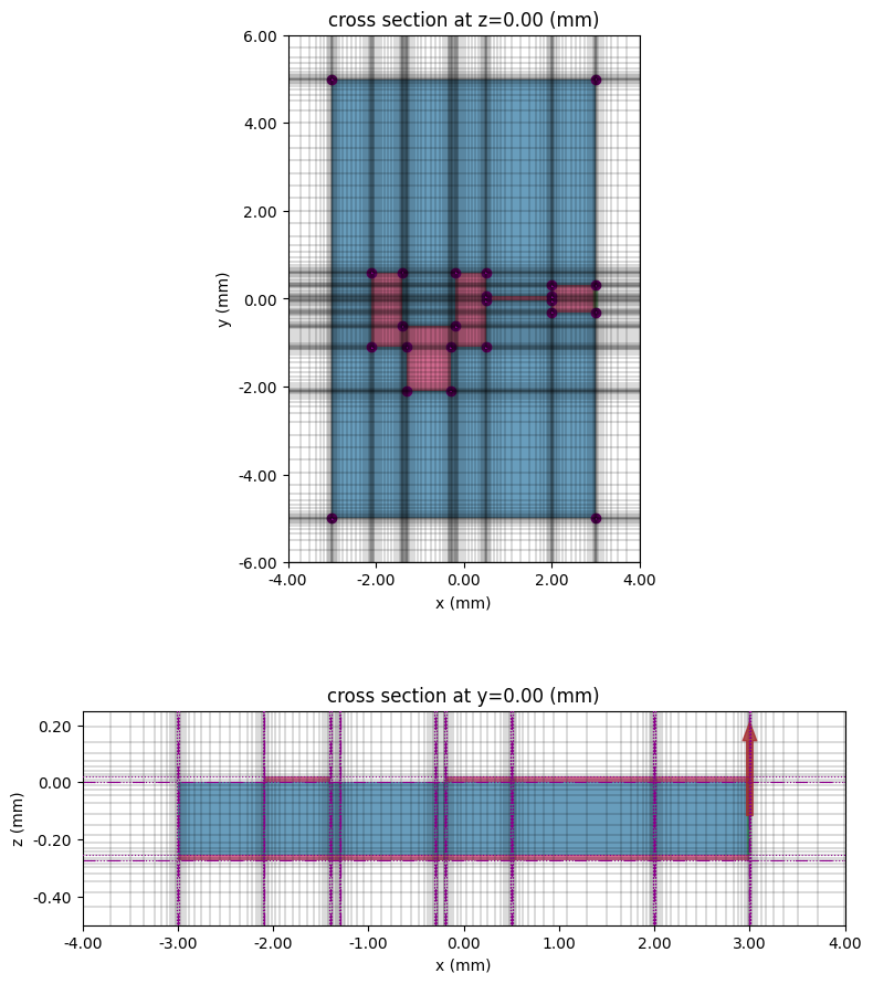
Before running, we should plot the simulation and check the grid.
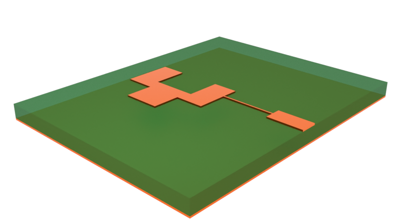
# Visualize the simulation in 3D (ports and radiation monitor not shown)
sim.plot_3d()
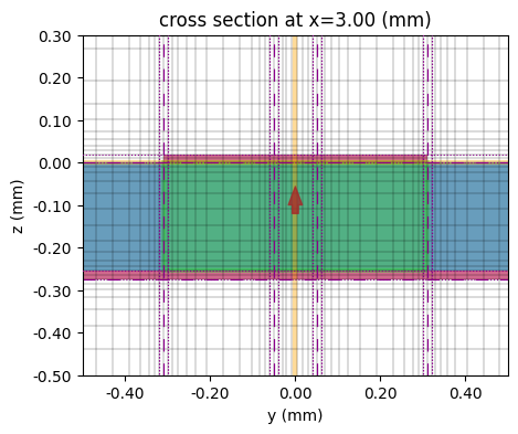
# Plot structures and grid at z=0 and y=0 cross sections
fig, ax = plt.subplots(2, 1, figsize=(8, 10), tight_layout=True)
tcm.plot_sim(z=0, ax=ax[0], monitor_alpha=0)
sim.plot_grid(z=0, ax=ax[0])
ax[0].set_xlim(-4 * mm, 4 * mm)
ax[0].set_ylim(-6 * mm, 6 * mm)
tcm.plot_sim(y=0, ax=ax[1], monitor_alpha=0)
sim.plot_grid(y=0, ax=ax[1])
ax[1].set_xlim(-4 * mm, 4 * mm)
ax[1].set_ylim(-0.5 * mm, 0.25 * mm)
ax[1].set_aspect(3)
plt.show()
# Plot lumped port
fig, ax = plt.subplots(figsize=(6, 4))
tcm.plot_sim(x=3 * mm, ax=ax)
sim.plot_grid(x=3 * mm, ax=ax)
ax.set_xlim(-0.5 * mm, 0.5 * mm)
ax.set_ylim(-0.5 * mm, 0.3 * mm)
plt.show()
Running the Simulation
Use tidy3d.web.upload() to upload the TCM job and get a cost estimation.
task_id = web.upload(tcm, task_name="edge_feed_tcm")
16:24:31 EST Created task 'edge_feed_tcm' with resource_id
             'sid-eb3565b8-07af-4753-b4e7-33659d5cb1ae' and task_type
             'TERMINAL_CM'.
             View task using web UI at
             'https://tidy3d.simulation.cloud/rf?taskId=pa-8c1d441d-73d2-4022-94
             00-2116fbc16f45'.
Task folder: 'default'.
16:24:40 EST Maximum FlexCredit cost: 0.429. Minimum cost depends on task
             execution details. Use 'web.real_cost(task_id)' after run.
The sequence of commands below starts the job, monitors progress, and downloads the results once it is finished.
# Run simulation
web.start(task_id)
web.monitor(task_id)
tcm_data = web.load(task_id)
16:24:41 EST Subtasks status - edge_feed_tcm
             Group ID: 'pa-8c1d441d-73d2-4022-9400-2116fbc16f45'
Batch status = preprocess
16:24:48 EST Batch status = running
16:26:05 EST Batch status = postprocess
16:26:18 EST Modeler has finished running successfully.
Billed flex credit cost: 0.240.
16:26:20 EST Loading component modeler data from cm_data.hdf5
The downloaded data is a TerminalComponentModelerData object. Use the smatrix() command to obtain the S-matrix.
# Calculate s-matrix
smat = tcm_data.smatrix()
Results
S-parameter
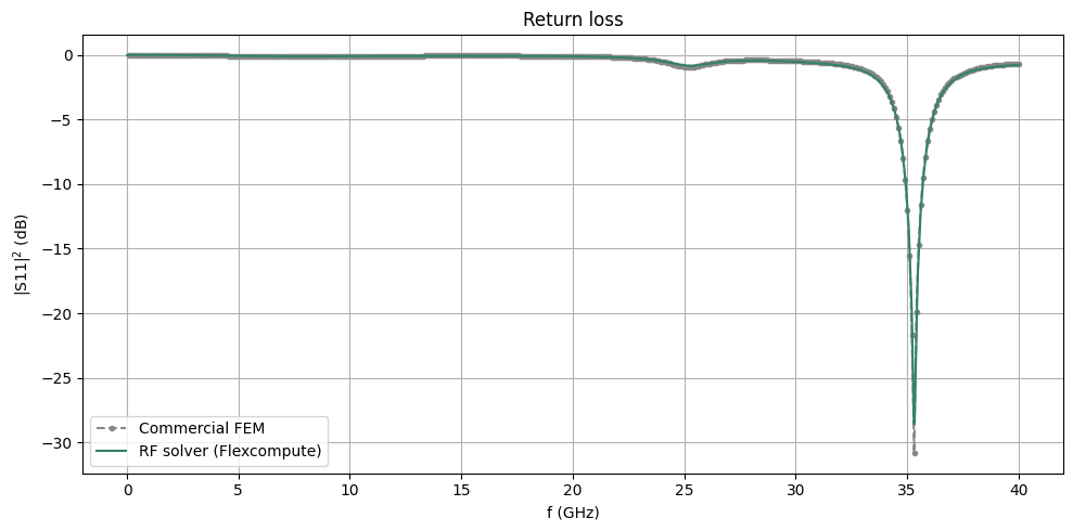
Below, we extract the simulated S11 and compare with the benchmark data. We observe good agreement.
# Extract S11 from smatrix
S11 = np.conjugate(smat.data.isel(port_in=0, port_out=0))
# Import benchmark data
freqs_fem, S11dB_fem = np.genfromtxt(
    "./misc/edge_feed_patch_fem.csv", delimiter=",", skip_header=1, unpack=True
)
# Plot S11 in dB
fig, ax = plt.subplots(figsize=(10, 5), tight_layout=True)
ax.plot(freqs_fem, S11dB_fem, "--.", color="#888888", label="Commercial FEM")
ax.plot(freqs / 1e9, 20 * np.log10(np.abs(S11)), color="#328362", label="RF solver (Flexcompute)")
ax.legend()
ax.grid()
ax.set_xlabel("f (GHz)")
ax.set_ylabel("|S11|$^2$ (dB)")
ax.set_title("Return loss")
plt.show()
Field profiles
To access the monitor data, we need to first load the SimulationData instance associated with the desired port excitation. This can be accessed using the appropriate key (the port name) on the dictionary stored in the data attribute of the TCM data.
# Access the simulation data for port 1 excitation
sim_data = tcm_data.data["LP1"]
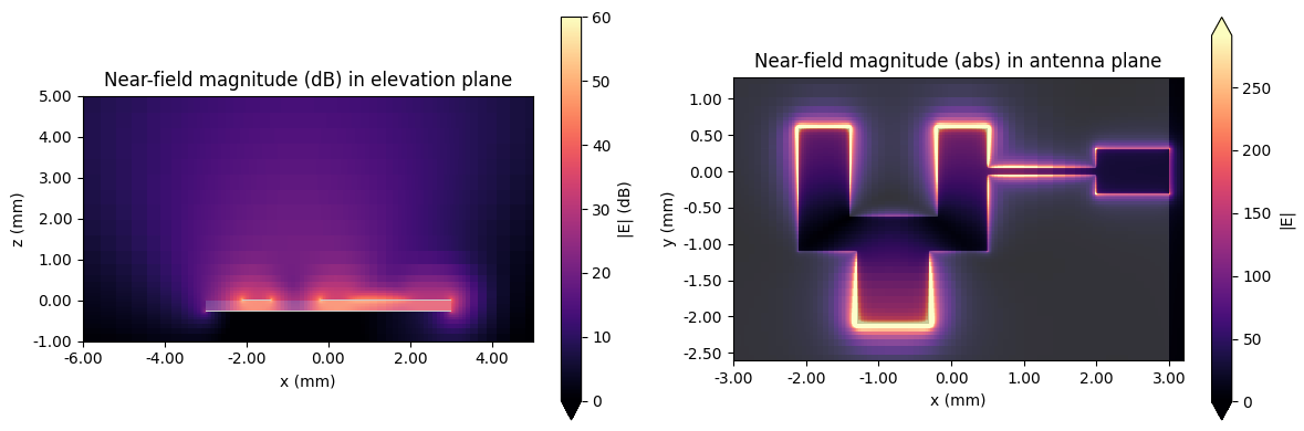
We plot the field profiles at f=f_target below.
# Visualize near-field profiles
fig, ax = plt.subplots(1, 2, figsize=(12, 4), tight_layout=True)
sim_data.plot_field(
    "xz plane", field_name="E", val="abs", scale="dB", f=f_target, ax=ax[0], vmax=60, vmin=0
)
ax[0].set_title("Near-field magnitude (dB) in elevation plane")
ax[0].set_xlim(-6 * mm, 5 * mm)
ax[0].set_ylim(-1 * mm, 5 * mm)
sim_data.plot_field("xy plane", field_name="E", val="abs", scale="lin", f=f_target, ax=ax[1])
ax[1].set_title("Near-field magnitude (abs) in antenna plane")
ax[1].set_xlim(-3 * mm, 3.2 * mm)
ax[1].set_ylim(-2.6 * mm, 1.3 * mm)
plt.show()
/home/dmarek/dev/custom_tidy/.venv/lib/python3.13/site-packages/xarray/computation/apply_ufunc.py:818: RuntimeWarning: divide by zero encountered in log10
  result_data = func(*input_data)
Antenna Gain
The get_antenna_metrics_data() method of the TCM data object calculates common antenna metrics provided a radiation monitor is defined. Below, we extract the gain data and compare it with benchmark data.
# Get antenna metrics from simulation data
antenna_metrics = tcm_data.get_antenna_metrics_data()

# Extract gain data
gain = antenna_metrics.gain
# Import and organize benchmark data
imp = np.genfromtxt("./misc/edge_feed_patch_fem_gain.csv", delimiter=",", skip_header=1)
phi_fem = np.unique(imp[:, 1]) / 180 * np.pi
theta_fem = np.unique(imp[:, 2]) / 180 * np.pi
gain_fem = xr.DataArray(
    np.reshape(imp[:, -1], (-1, 91)), coords={"phi": phi_fem, "theta": theta_fem}
)
Below is a convenience function that collects the gain data for forward and backward directions (phi and phi-180 degrees) into a single array. We need to do this because the elevation angle theta ranges between (0, 180) degrees whereas the azimuthal angle phi ranges between (-180, 180) degrees.
def get_full_elevation_plane_data(data, phi_forward, phi_backward):
    """Get full elevation plane data for given phi (azimuth) forward and backward angle"""
    # Assemble full theta (elevation angle) coordinate
    thetas = data.theta
    thetas_full = np.unique(np.append(-thetas, thetas))

    # Assemble data
    data_forward = data.sel(phi=phi_forward, method="nearest").squeeze()
    data_backward = data.sel(phi=phi_backward, method="nearest").squeeze()
    data_full = np.append(data_backward[:0:-1], data_forward)

    return thetas_full, data_full
The gain data for the elevation planes phi=0 degrees and phi=90 degrees are collected below.
# Get gain in the elevation plane for phi = 0 and 90 degrees
theta_elev, gain_elev = get_full_elevation_plane_data(gain, phi_forward=0, phi_backward=-np.pi)
_, gain_elev_90 = get_full_elevation_plane_data(
    gain, phi_forward=np.pi / 2, phi_backward=-np.pi / 2
)

# Get same data for benchmark dataset
_, gain_elev_fem = get_full_elevation_plane_data(gain_fem, phi_forward=0, phi_backward=-np.pi)
_, gain_elev_fem_90 = get_full_elevation_plane_data(
    gain_fem, phi_forward=np.pi / 2, phi_backward=-np.pi / 2
)
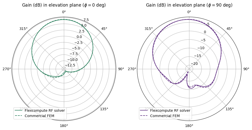
We plot the gain comparison below.
# Gain comparison plot
fig, ax = plt.subplots(1, 2, figsize=(10, 8), tight_layout=True, subplot_kw={"projection": "polar"})

# Plot gain for phi =0
ax[0].plot(theta_elev, 10 * np.log10(gain_elev), color="#328362", label="Flexcompute RF solver")
ax[0].plot(theta_elev, 10 * np.log10(gain_elev_fem), "--", color="#328362", label="Commercial FEM")
ax[0].set_title("Gain (dB) in elevation plane ($\\phi=0$ deg)", pad=30)

# Plot gain for phi = 90deg
ax[1].plot(theta_elev, 10 * np.log10(gain_elev_90), color="#623283", label="Flexcompute RF solver")
ax[1].plot(
    theta_elev, 10 * np.log10(gain_elev_fem_90), "--", color="#623283", label="Commercial FEM"
)
ax[1].set_title("Gain (dB) in elevation plane ($\\phi=90$ deg)", pad=30)

for axis in ax:
    axis.set_theta_direction(-1)
    axis.set_theta_offset(np.pi / 2.0)
    axis.legend()

plt.show()
The LobeMeasurer is a Tidy3D plugin tool that automatically calculates lobe measurements based on a radiation profile.
# Calculate radiation lobe properties
lobes = rf.LobeMeasurer(angle=theta_elev, radiation_pattern=gain_elev, apply_cyclic_extension=False)
lobes_fem = rf.LobeMeasurer(
    angle=theta_elev, radiation_pattern=gain_elev_fem, apply_cyclic_extension=False
)
The properties of the main lobe are reported below. Angle units are radians. In addition to the main_lobe property, users can also view lobe_measures for a summary table of all detected lobes, side_lobes for side lobe properties, and sidelobe_level.
# Report main lobe properties
lobes.main_lobe
direction                                                  -0.0
magnitude                                              4.710105
beamwidth                                               1.46851
beamwidth magnitude                                    2.355052
beamwidth bounds       (-0.7808736288572525, 0.687636833974749)
FNBW                                                        NaN
FNBW bounds                                          (nan, nan)
Name: 0, dtype: object
The main lobe is compared between the RF solver and the benchmark.
print(
    f"RF solver: The main lobe is at theta = {lobes.main_lobe.direction / np.pi * 180:.0f} degrees, magnitude = {lobes.main_lobe.magnitude:.1f}, and beamwidth = {lobes.main_lobe.beamwidth / np.pi * 180:.0f} degrees"
)
RF solver: The main lobe is at theta = -0 degrees, magnitude = 4.7, and beamwidth = 84 degrees
print(
    f"FEM benchmark: The main lobe is at theta = {lobes_fem.main_lobe.direction / np.pi * 180:.0f} degrees, magnitude = {lobes_fem.main_lobe.magnitude:.1f}, and beamwidth = {lobes_fem.main_lobe.beamwidth / np.pi * 180:.0f} degrees"
)
FEM benchmark: The main lobe is at theta = -0 degrees, magnitude = 4.8, and beamwidth = 83 degrees
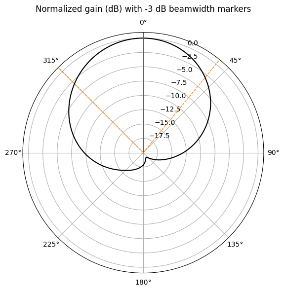
The LobeMeasurer.plot() method automatically adds markers to indicate main lobe direction and -3 dB beamwidth. This is demonstrated below.
# Gain comparison plot
fig, ax = plt.subplots(figsize=(6, 6), tight_layout=True, subplot_kw={"projection": "polar"})
ax.set_theta_direction(-1)
ax.set_theta_offset(np.pi / 2.0)

# Plot gain for phi =0
ax.plot(theta_elev, 10 * np.log10(gain_elev / np.max(gain_elev)), color="black")
lobes.plot(lobe_index=0, ax=ax)
ax.set_ylim(-20, 1)
ax.set_title("Normalized gain (dB) with -3 dB beamwidth markers", pad=30)
plt.show()
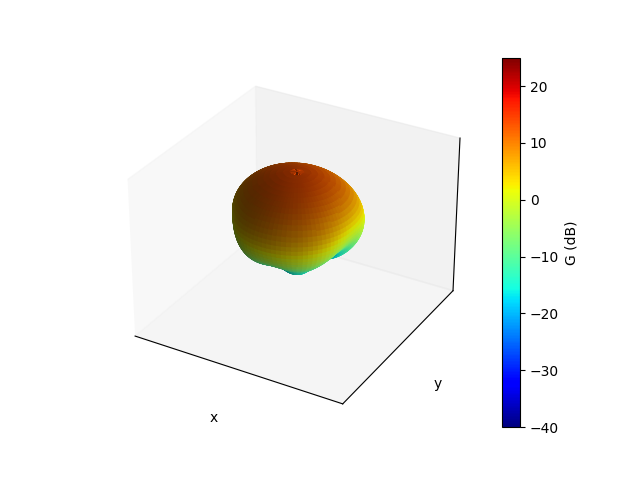
3D Radiation Pattern
In this section, we demonstrate how to plot the radiation pattern in 3D. The ipympl library enables interactive plots so that we can rotate the 3D plot with the mouse cursor. (This function is only available in a Jupyter notebook and does not work on the browser.)
# Activate interactive plotting for 3D radiation pattern
# Requires ipympl library to be installed (comment line below if requirement not met)
%matplotlib widget
# Create figure and axes
fig_3d = plt.figure()
ax_3d = fig_3d.add_subplot(1, 1, 1, projection="3d")
limits = 1.0
ax_3d.set_xlim(-limits, limits)
ax_3d.set_ylim(-limits, limits)
ax_3d.set_zlim(-limits, limits)
ax_3d.set_xticks([])
ax_3d.set_yticks([])
ax_3d.set_zticks([])
ax_3d.set_xlabel("x")
ax_3d.set_ylabel("y")
ax_3d.set_zlabel("z")

# Rescale gain according to max and min dB values
dB_min, dB_max = (-40, 25)
G = 20 * np.log10(np.abs(gain.squeeze()))
G_scaled = np.clip((G - dB_min) / (dB_max - dB_min), a_min=0, a_max=1)

# Create 3D dataset according to scaled gain
phi_s, theta_s = np.meshgrid(phi, theta)
X = G_scaled * np.cos(phi_s) * np.sin(theta_s)
Y = G_scaled * np.sin(phi_s) * np.sin(theta_s)
Z = G_scaled * np.cos(theta_s)

# Select color map
color_map = plt.cm.jet

# Plot surface
surf = ax_3d.plot_surface(
    X,
    Y,
    Z,
    cstride=2,
    rstride=2,
    facecolors=color_map(G_scaled),
)

# Plot color bar
cbar = fig_3d.colorbar(
    plt.cm.ScalarMappable(norm=colors.Normalize(vmax=dB_max, vmin=dB_min), cmap=color_map),
    ax=ax_3d,
    label="G (dB)",
)
plt.show()
# Close 3D figure and deactivate interactive plotting
plt.close(fig_3d)
%matplotlib inline
Lowering Simulation Cost
For benchmark purposes, we used a relatively fine simulation grid. Users might wish to make the grid coarser in order to save on computation costs, particularly if they are still in the design iteration process. In this section, we demonstrate that using a coarser grid can save significantly on cost with a relatively minor compromise to accuracy.
Reducing Grid Resolution
The main changes are that we reduced min_steps_along_axis to 1 and increased the size of dl in the corner_refinement setting.
def create_layer_refinement_coarse(structure_list):
    """Create predefined layer refinement spec from input structure list"""
    return rf.LayerRefinementSpec.from_structures(
        structures=structure_list,
        min_steps_along_axis=1,
        corner_refinement=td.GridRefinement(dl=2 * t, num_cells=2),
    )


lr3 = create_layer_refinement_coarse([str_gnd])
lr4 = create_layer_refinement_coarse([str_feed1, str_feed2, str_ant])

# Define grid spec
gspec_coarse = td.GridSpec.auto(
    wavelength=td.C_0 / f_target,
    min_steps_per_wvl=20,
    layer_refinement_specs=[lr3, lr4],
)
# Copy new sim and TCM from previous
sim_coarse = sim.updated_copy(grid_spec=gspec_coarse)
tcm_coarse = tcm.updated_copy(simulation=sim_coarse)
We run the simulation below.
tcm_coarse_data = web.run(tcm_coarse, task_name="tcm_coarse")
smat_coarse = tcm_coarse_data.smatrix()
16:26:23 EST Created task 'tcm_coarse' with resource_id
             'sid-675e121b-7ee2-4fa7-a7a1-f3f267e1ce4b' and task_type
             'TERMINAL_CM'.
             View task using web UI at
             'https://tidy3d.simulation.cloud/rf?taskId=pa-1a6b3be2-9e9c-45d7-ba
             57-c69a9a72eeeb'.
Task folder: 'default'.
16:26:30 EST Maximum FlexCredit cost: 0.057. Minimum cost depends on task
             execution details. Use 'web.real_cost(task_id)' after run.
16:26:31 EST Subtasks status - tcm_coarse
             Group ID: 'pa-1a6b3be2-9e9c-45d7-ba57-c69a9a72eeeb'
Batch status = preprocess
16:26:37 EST Batch status = running
16:27:40 EST Batch status = postprocess
16:27:50 EST Modeler has finished running successfully.
16:27:51 EST Billed flex credit cost: 0.057.
16:27:52 EST Loading component modeler data from cm_data.hdf5
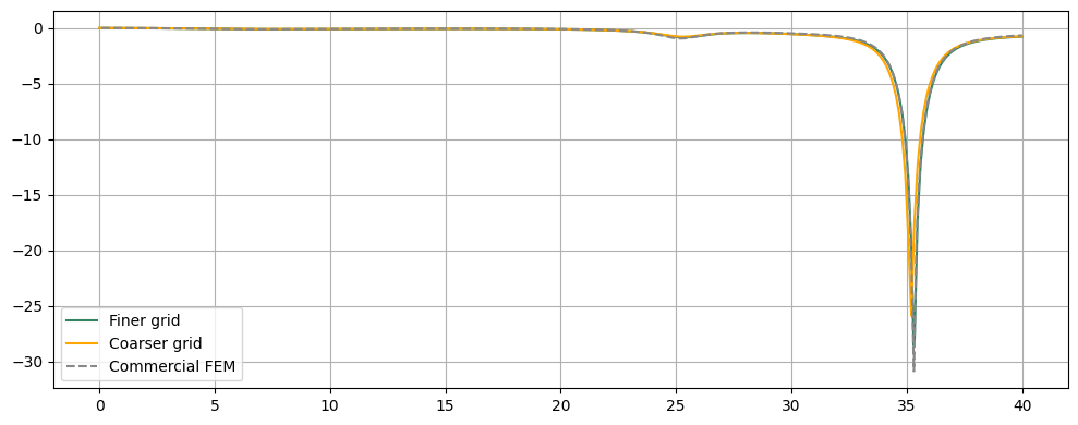
Comparing Performance
The S-parameter and antenna gain profile are compared below. We observe a relatively minor accuracy reduction for the cheaper simulation, making it suitable for rapid iteration during the initial stages of a component design process.
# Compare S-parameter between finer and coarser grid simulations
S11_coarse = np.conjugate(smat_coarse.data.isel(port_in=0, port_out=0))

fig, ax = plt.subplots(figsize=(10, 4), tight_layout=True)
ax.plot(freqs / 1e9, 20 * np.log10(np.abs(S11)), color="#328362", label="Finer grid")
ax.plot(freqs / 1e9, 20 * np.log10(np.abs(S11_coarse)), color="orange", label="Coarser grid")
ax.plot(freqs_fem, S11dB_fem, "--", color="#888888", label="Commercial FEM")
ax.legend()
ax.grid()
plt.show()
# Compare antenna gain between finer and coarser grid simulations
antenna_metrics_coarse = tcm_coarse_data.get_antenna_metrics_data()
gain_coarse = antenna_metrics_coarse.gain
# Get gain in the elevation plane for phi = 0 and 90 degrees
_, gain_elev_coarse = get_full_elevation_plane_data(gain_coarse, phi_forward=0, phi_backward=-np.pi)
_, gain_elev_coarse_90 = get_full_elevation_plane_data(
    gain_coarse, phi_forward=np.pi / 2, phi_backward=-np.pi / 2
)
# Gain comparison plot
fig, ax = plt.subplots(1, 2, figsize=(10, 8), tight_layout=True, subplot_kw={"projection": "polar"})

# Plot gain for phi =0
ax[0].plot(theta_elev, 10 * np.log10(gain_elev), color="#328362", label="Finer grid")
ax[0].plot(theta_elev, 10 * np.log10(gain_elev_coarse), color="orange", label="Coarser grid")
ax[0].plot(theta_elev, 10 * np.log10(gain_elev_fem), "--", color="#888888", label="Commercial FEM")
ax[0].set_title("Gain (dB) in elevation plane ($\\phi=0$ deg)", pad=30)

# Plot gain for phi = 90deg
ax[1].plot(theta_elev, 10 * np.log10(gain_elev_90), color="#328362", label="Finer grid")
ax[1].plot(theta_elev, 10 * np.log10(gain_elev_coarse_90), color="orange", label="Coarser grid")
ax[1].plot(
    theta_elev, 10 * np.log10(gain_elev_fem_90), "--", color="#888888", label="Commercial FEM"
)
ax[1].set_title("Gain (dB) in elevation plane ($\\phi=90$ deg)", pad=30)

for axis in ax:
    axis.set_theta_direction(-1)
    axis.set_theta_offset(np.pi / 2.0)
    axis.legend()

plt.show()
Reference
[1] Khan, J., Ullah, S., Ali, U., Tahir, F. A., Peter, I., & Matekovits, L. (2022). Design of a Millimeter-Wave MIMO Antenna Array for 5G Communication Terminals. Sensors, 22(7), 2768.