How to Design an Airplane, Build a 3D Model, and Perform RANS CFD in 30 Minutes
In this article, we illustrate a typical workflow of using XFoil, Engineering Sketch Pad (ESP), Pointwise, and Flow360 to analyze the aerodynamic performance of a wing-body configuration. The goal is to perform RANS simulations of several airplane models, each with a wing and a fuselage, and to compute the drag and induced flow downstream of the airplanes. In less than half an hour, one can go from a pure concept to concrete CFD solutions, with outputs ranging from key quantities of interest to surface pressure and streamlines, and to detailed three-dimensional flow fields.
The process starts with two-dimensional design with Xfoil, which takes 5 minutes with some familiarity with Xfoil. It then proceeds to the construction of a three dimensional model, which also takes 5 minutes if one is proficient with ESP. The next step in the process is meshing, which takes about 5 minutes of human time – no geometry cleanup required – and another 3 minutes of computer time. Finally, uploading the mesh and running the simulation with Flow360 can take less than 5 minutes with a good Internet connection and familiarity with the Flow360 web UI.
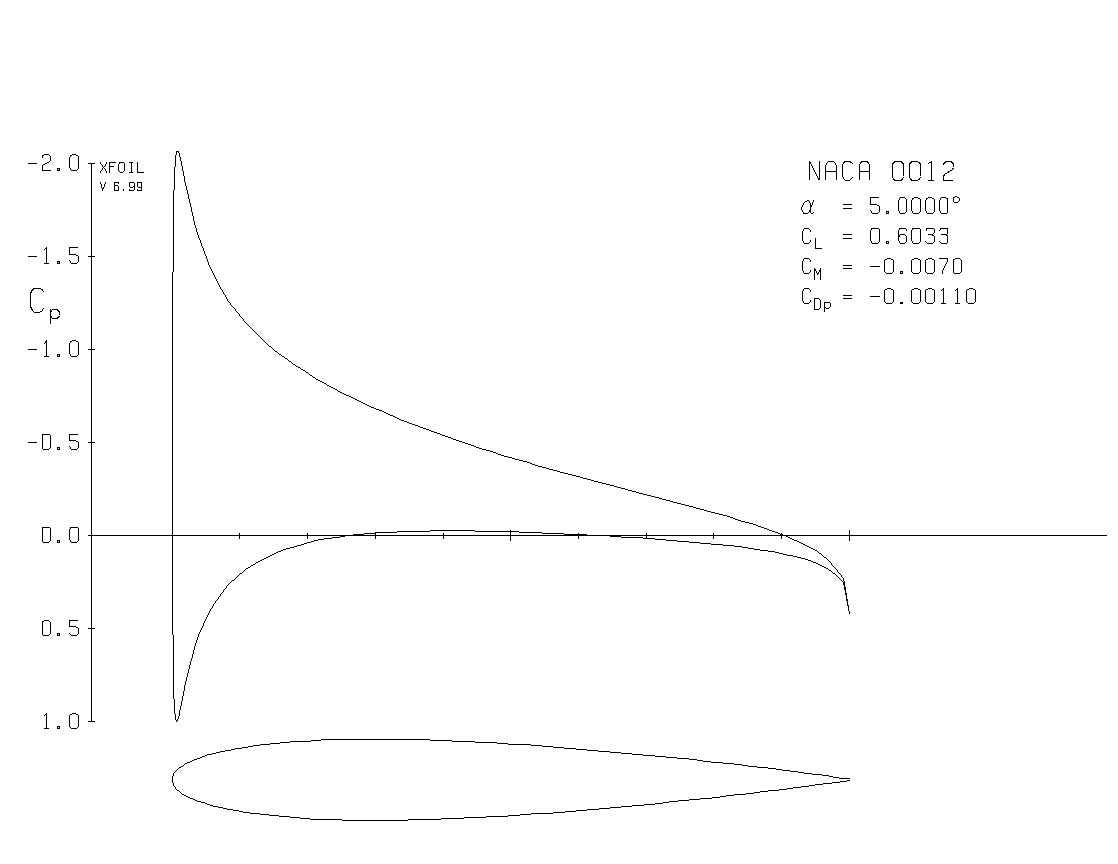
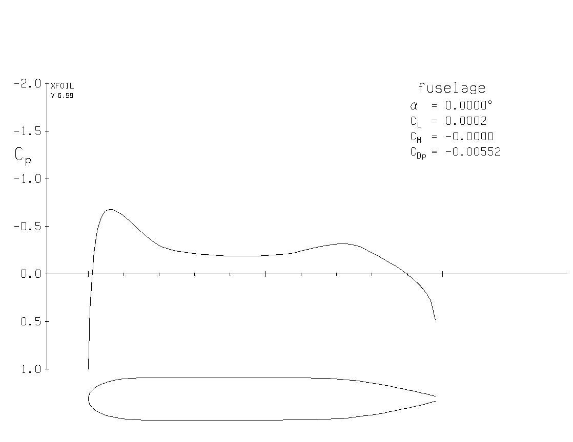
The first step is to design the airfoil used in the wing and the fuselage geometry. Here we use the NACA 0012 airfoil for the wing. We extend the maximum thickness of a NACA 0024 airfoil horizontally to make the fuselage shape, as shown below. For how to use the open source software XFoil to design airfoils, please refer to its documentation at XFoil Subsonic Airfoil Development System
The next step is to construct a three-dimensional geometry using Engineering Sketch Pad (ESP). We used the REVOLVE command to make the fuselage from the two-dimensional cross section, Each airfoil section is scaled and translated into its respective position. Note that we extended the chord around the wing-fuselage junction, a simple method to reduce junction flow separation. The smooth airfoil is split into upper and lower surfaces, each represented using a SPLINE. The blunt trailing edge is represented by a line segment. The resulting series of closed contours are formed into a half-wing using the BLEND command. The other half wing is then constructed using the MIRROR command. The fuselage and both wings are then joined into an airplane using the UNION command. For how to use ESP to construct 3D models, please refer to the examples and documentation at Engineering Sketch Pad (ESP)
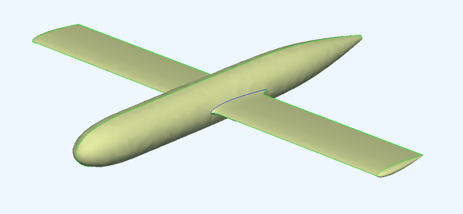
The resulting model is saved into an EGADS file and imported into Pointwise. Typically, no geometry clean-up is necessary with the EGADS format. We then use Flashpoint, an automatic surface generation tool, to generate the surface mesh. We set the maximum aspect ratio to 50 and turn refinement off at concave edges to obtain good mesh around trailing edges. For more information on the Flashpoint feature of Pointwise, please refer to Mesh and Run a High-Fidelity Aircraft Simulation in Minutes
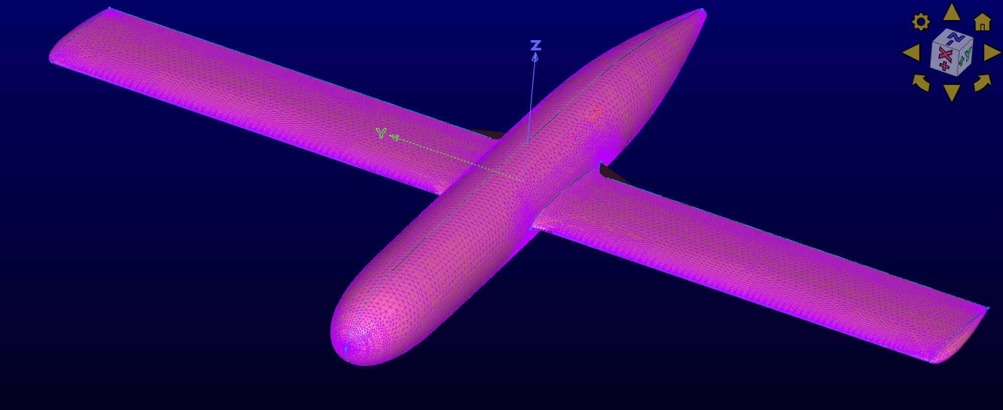
To generate the volume mesh, we first create a spherical mesh with a radius 100 times the length of the airplane. This spherical mesh serves as the far-field. We then create a block in the space between the far-field mesh and the airplane surface mesh. We add a box-shaped source behind the wing to resolve the induced flow. Volume mesh is then generated using the TRex algorithm, the first layer thickness on the wall set to one-millionth the length of the airplane. Before saving the mesh into the CGNS format, we name the airplane and far-field with different boundary conditions. For more information on how to use Pointwise, please refer to Pointwise
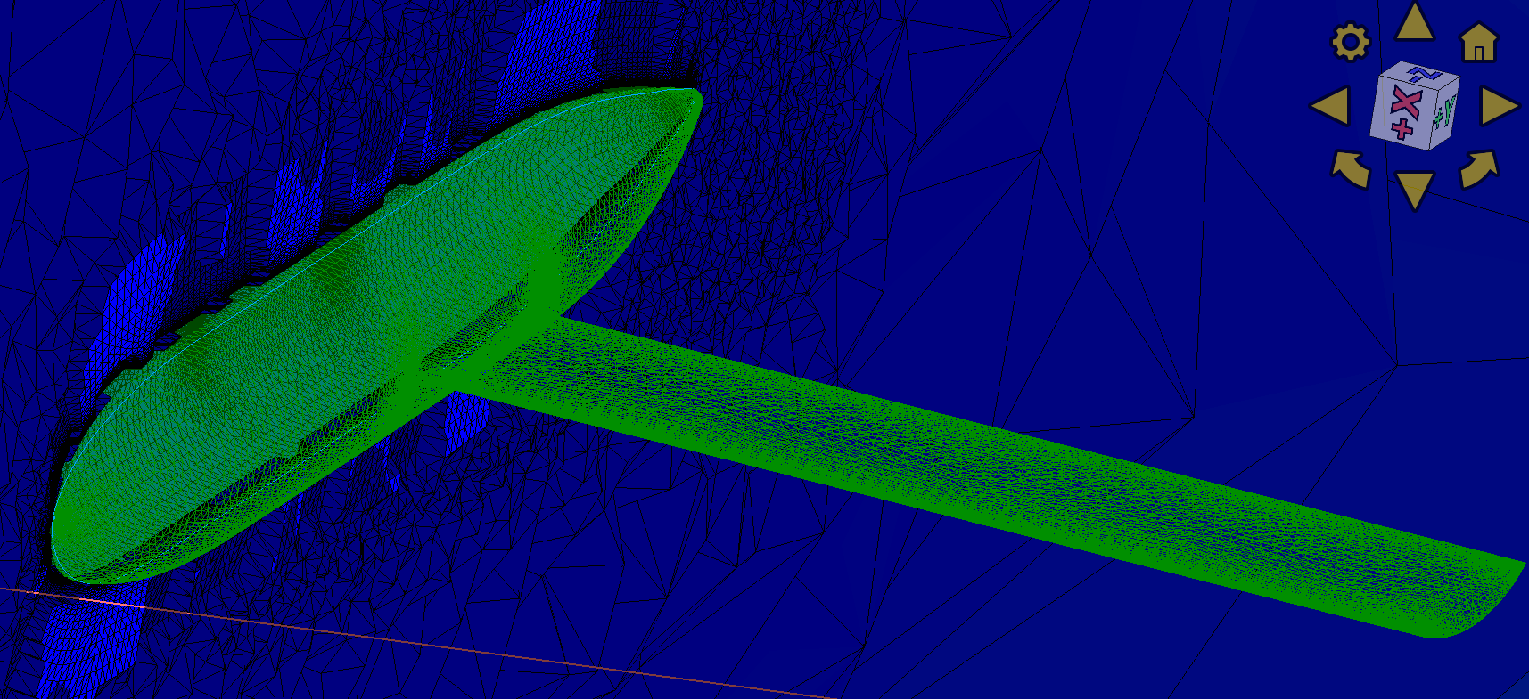
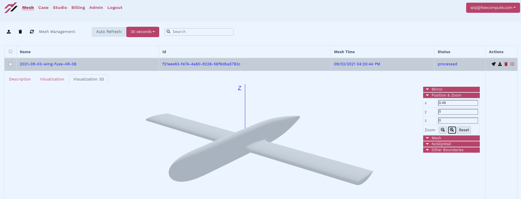
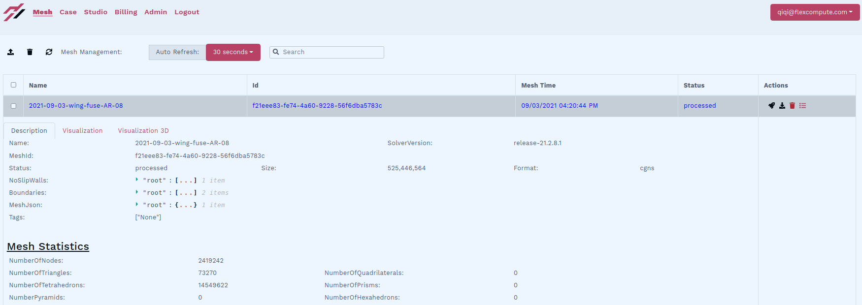
We then upload the mesh to the Flow360 website. After the mesh is processed, we see on the webpage that the mesh contains about 2.4 million nodes and about 14.5 million tetrahedrons. In the visualization tab, we confirm the correct mesh is uploaded by inspecting the surfaces.
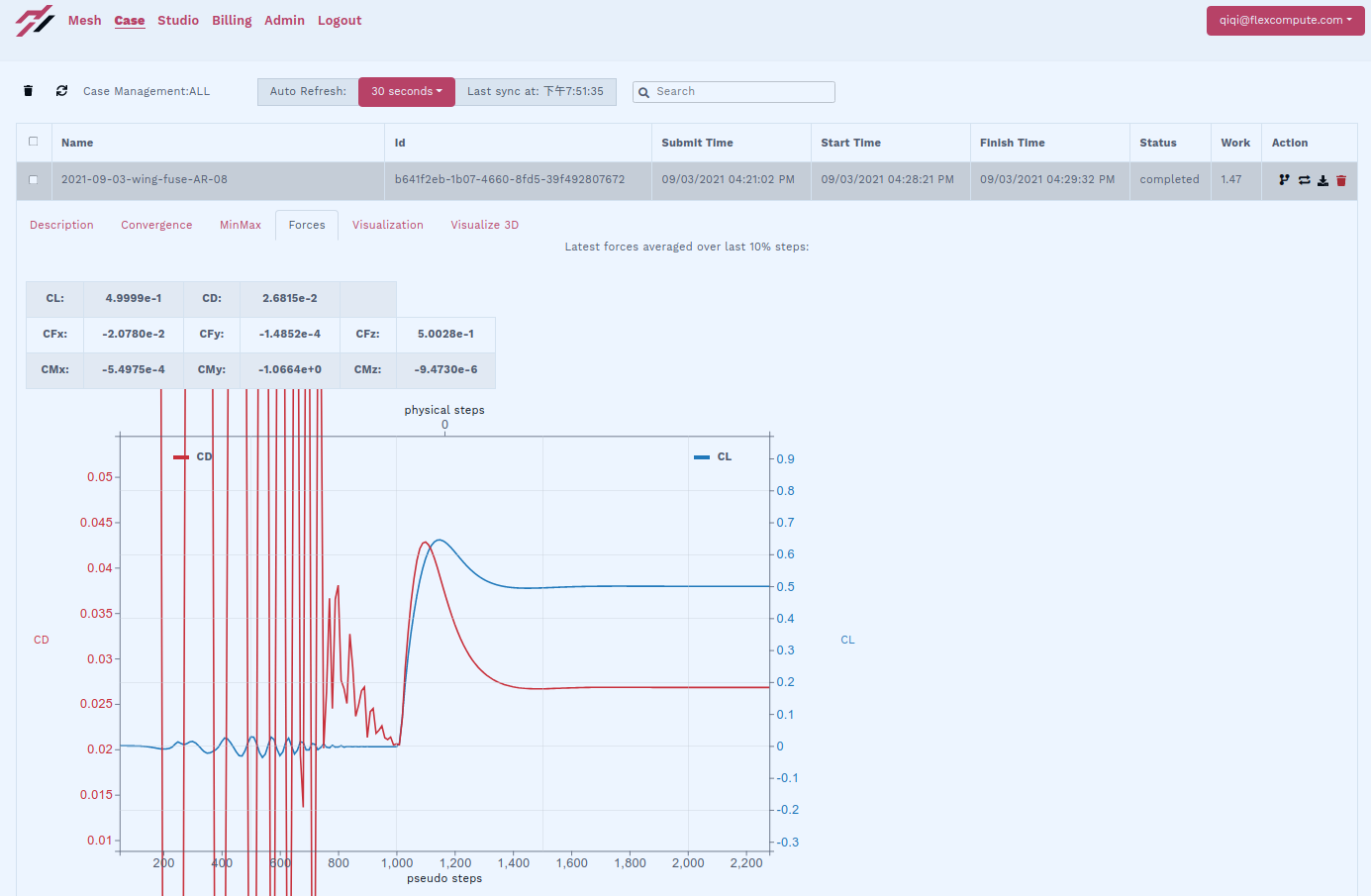
We then launch a Flow360 case from the mesh. We specify a Mach number of 0.3, a Reynolds number of about ten million, and a target lift coefficient of 0.5. The simulation converged in slightly more than one minute. It took over two thousand steps to converge the mass conservation, momentum conservation, and energy conservation equations to the default tolerance 1E-10. It is worth noting that the angle of attack is automatically adjusted starting from the 1000th iteration in order to match the target lift coefficient of 0.5. For more information about how to set up a simulation in Flow360, please refer to Flow360 Documentation
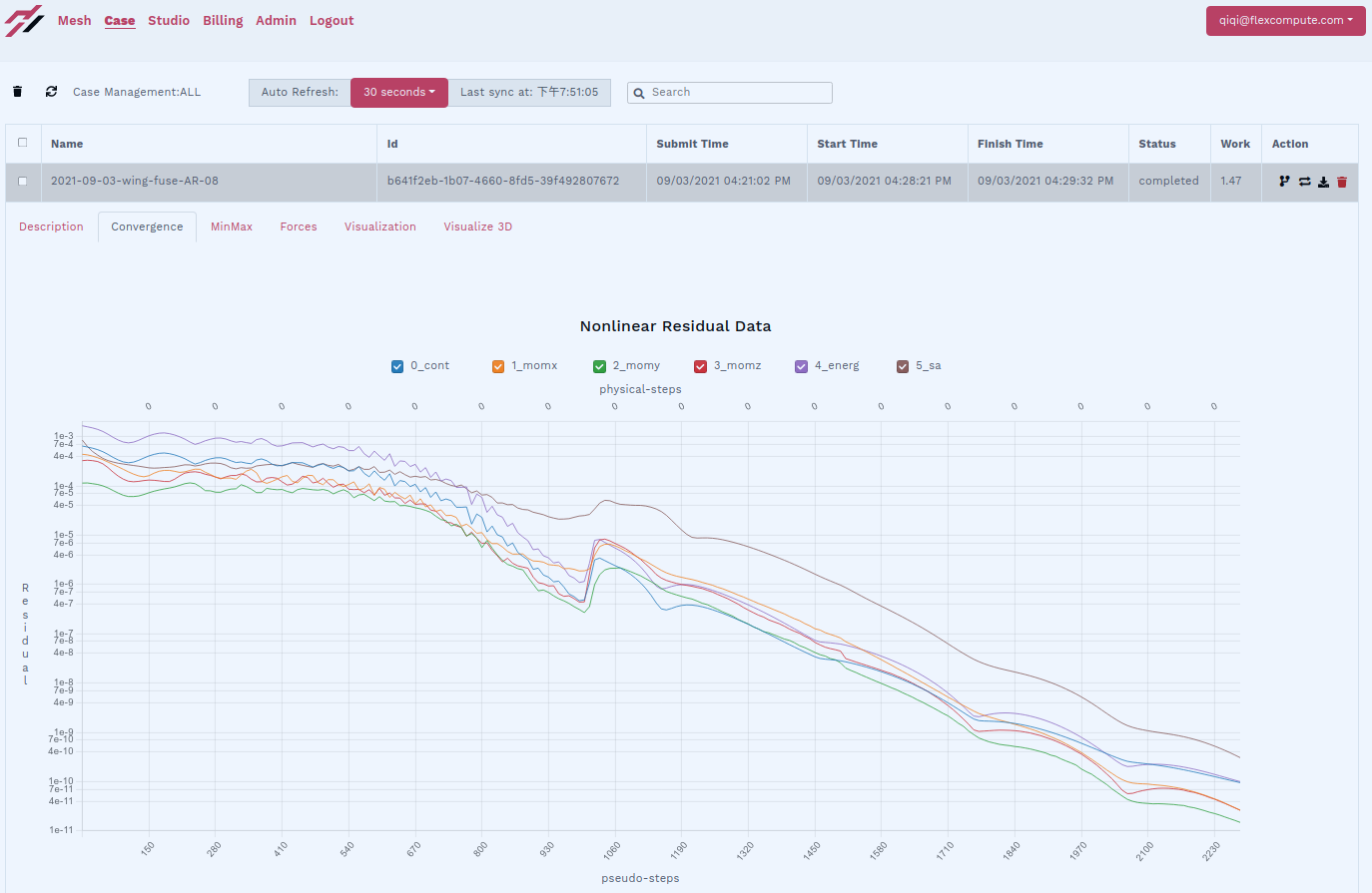
The convergence history of the lift and drag coefficients can also be observed from the Flow360 website, both during the simulation and after it completes. We see that the lift reaches the target of 0.5, and the drag coefficient converges to 0.0268. The convergence of other forces and moments is also displayed.
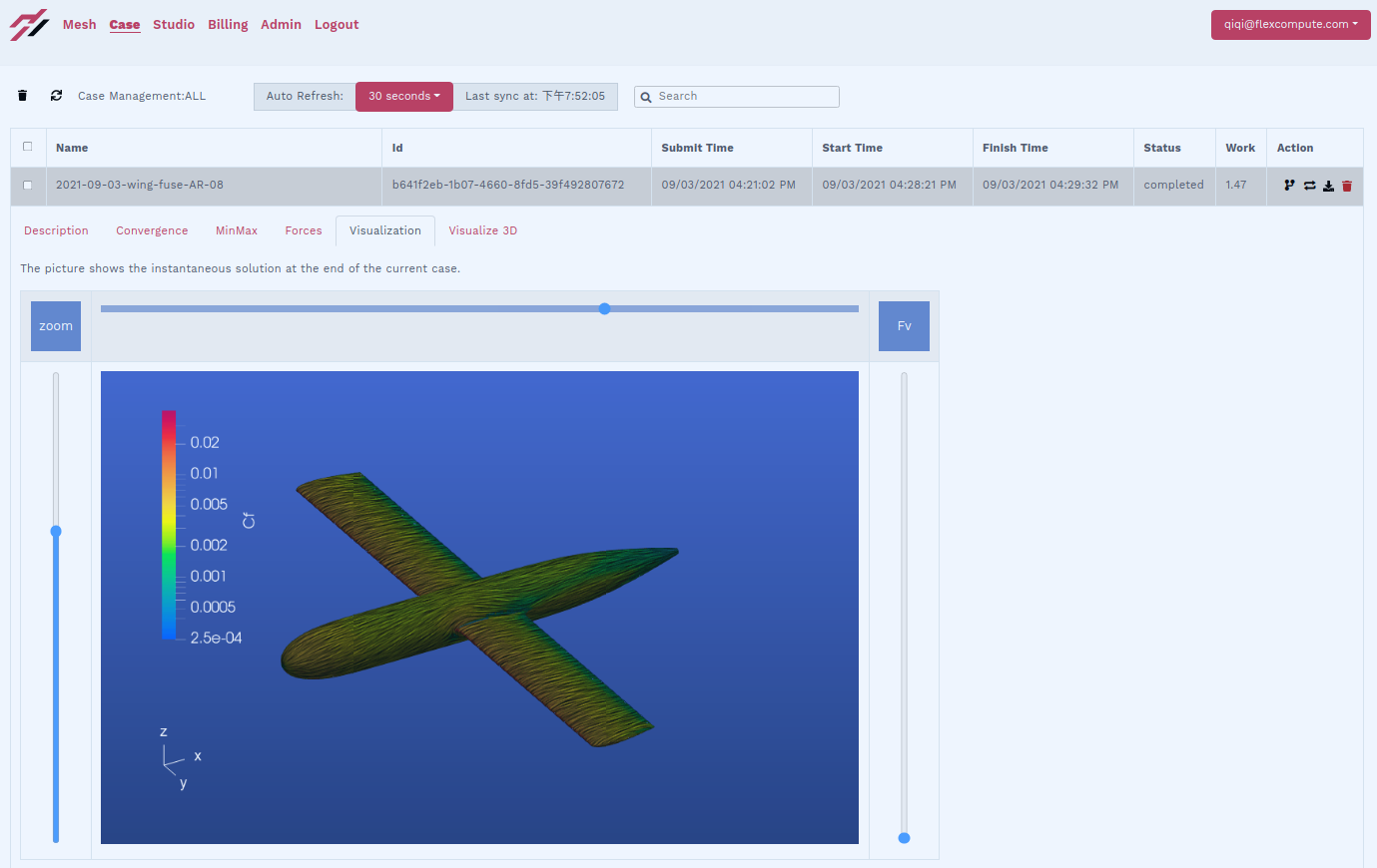
After the simulation completes, we can inspect the surface flow field by clicking the visualization tab on the Flow360 website. The surface streamlines show attached flow both on the wing and on the fuselage.
The pressure coefficient can also be visualized on the webpage.
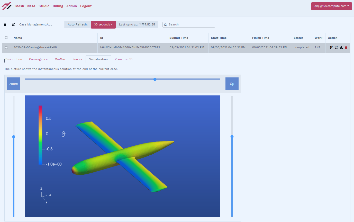
The above workflow can be easily automated by simple scripting. We use such automation to build, mesh, and simulate several airplanes of different aspect ratios: 3, 5, and 8. The pictures above correspond to an aspect ratio of 8. The following pictures show the web-based pressure coefficient visualization for the lower aspect ratios, with the same nominal wing area.
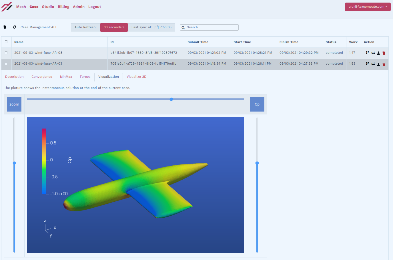
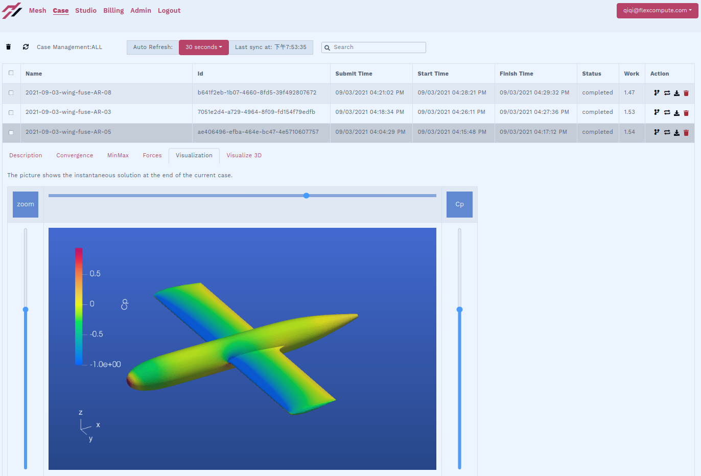
To examine more details of the simulation, we can click the “download” button on each completed case for the visualization files, available in Tecplot and Paraview formats. These files contain the entire flow field. The following figures show the Z-velocity on a plane 20% airplane lengths after the tail. For more information about using Tecplot for flow visualization, please refer to Tecplot
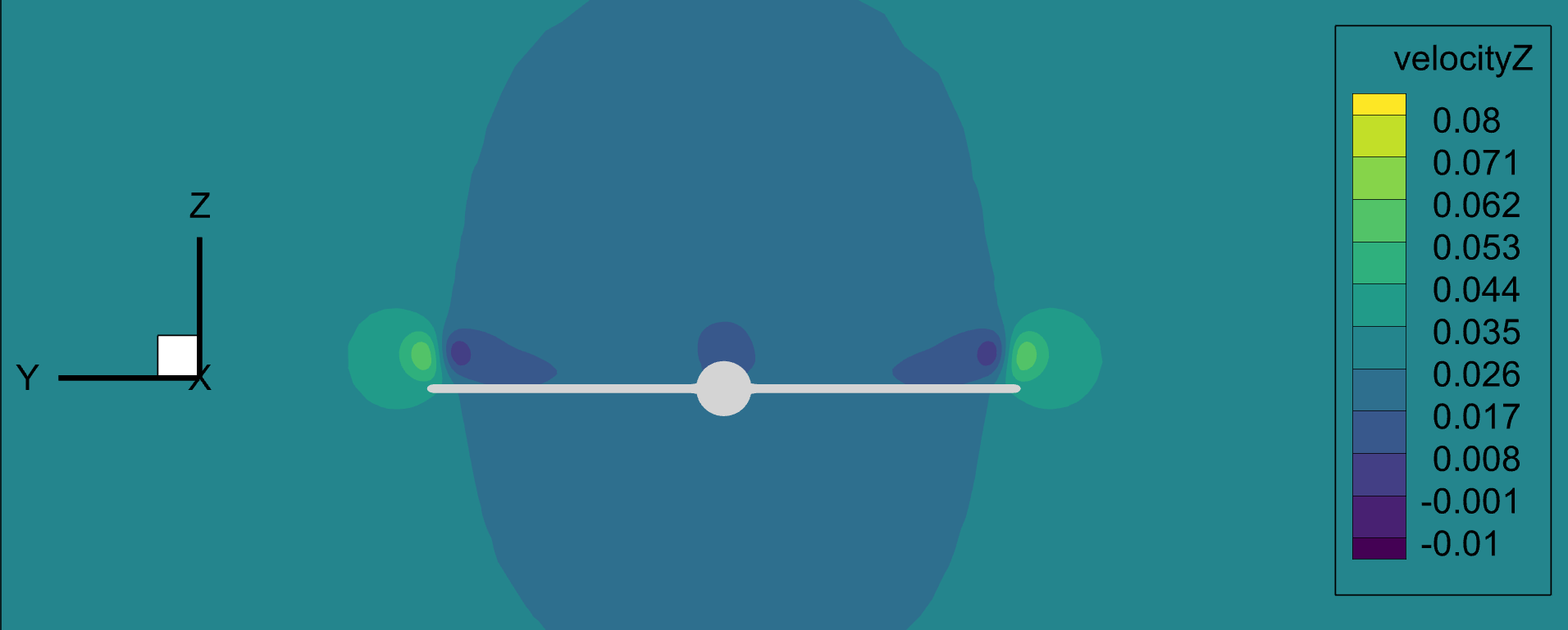
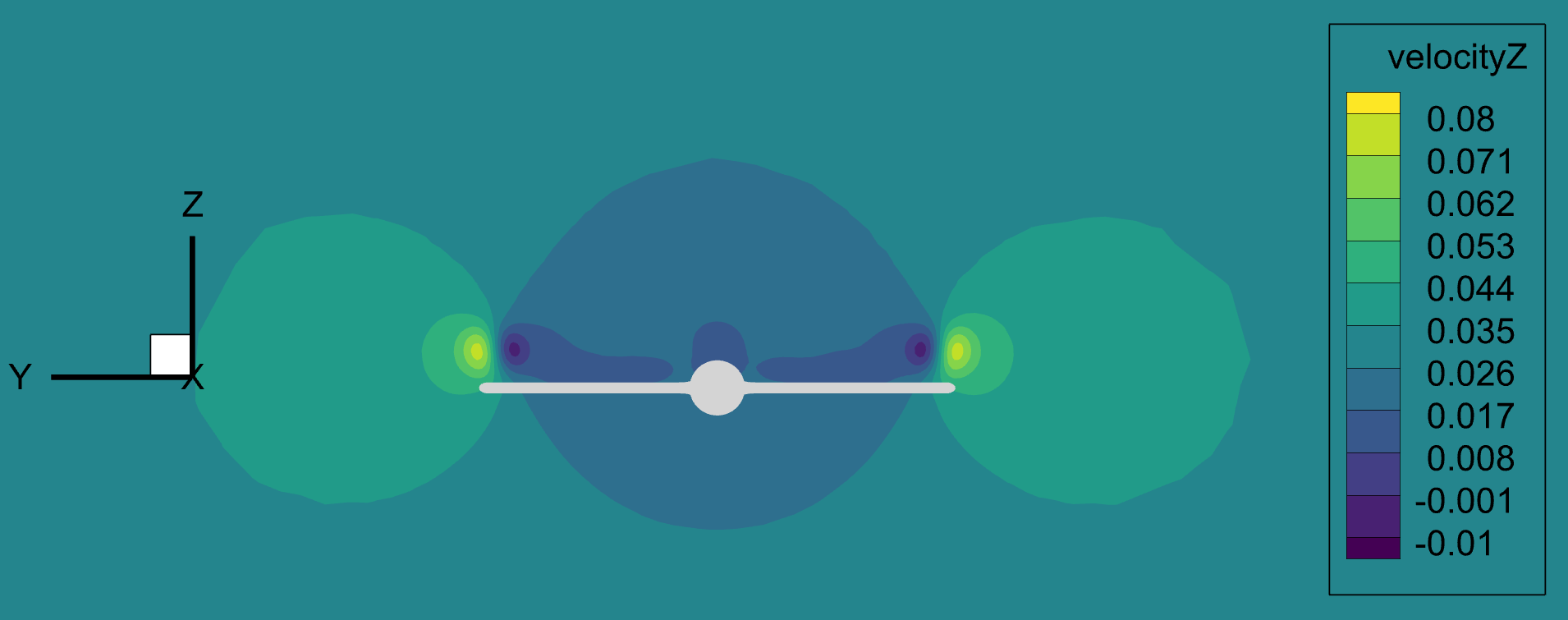
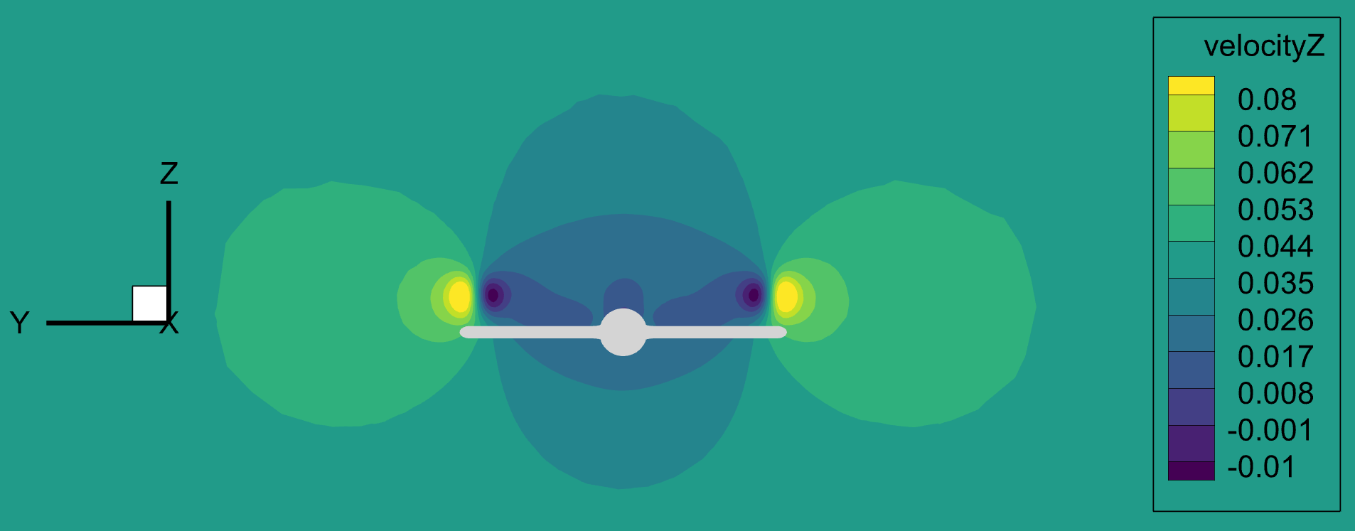
The wingtip vortices and induced flow are clearly visible. Although the three airplanes generate identical lift forces, the tip vortices and induced flow are clearly stronger for the lower aspect ratio wings. This is reflected in the drag coefficients. All three airplanes achieve the same lift coefficient of 0.5 with identical reference areas. The drag coefficients computed by Flow360 are 2.6815e-2, 3.2031e-2, and 4.1975e-2, respectively, for the airplanes of decreasing aspect ratios.
The entire process from concept to CFD solution takes less than half an hour for a proficient engineer, and much less than that if the components are automated by scripting, which is supported in ESP, Pointwise, and Flow360. Such a fast and automatable workflow can dramatically accelerate the design iteration cycle of your aerospace vehicles.


