TIDY3D
FDTD AND MORE


Python FDTD
Tidy3D provides a rich Python interface for defining and running FDTD simulations. Python is used for setting up and analyzing simulation results. The FDTD algorithm runs in the background on Flexcompute's servers, which are highly optimized for solving FDTD efficiently.
If you do not wish to install, please click this button to get started quickly.
Run this Python codeSet up and run your first FDTD simulation
With just a few steps, you can set up and run your first FDTD simulation using the Python user interface. Additionally, you may want to explore other examples and tutorials to create your own simulations.
3. Analyze results
ax = sim_data.plot_field("fields", "Ey", z=0)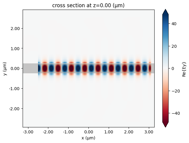
How well does python FDTD perform
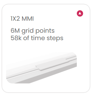
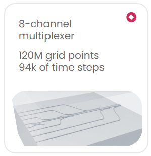
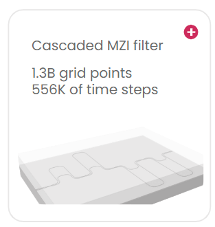
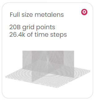
Tidy3D consistently outperforms other conventional FDTD solvers by an order of 100x or more. We achieve this performance improvement through the use of our custom hardware, which is optimized specifically for large scale FDTD simulation. As such, simulations that may take several hours or days on conventional hardware may be done in just minutes using Tidy3D. Furthermore, we can handle simulations with several billions of spatial degrees of freedom, which require too much memory to handle using conventional FDTD solvers.
For more details, see our papers and examples.
 40s
40s
 3min 40s
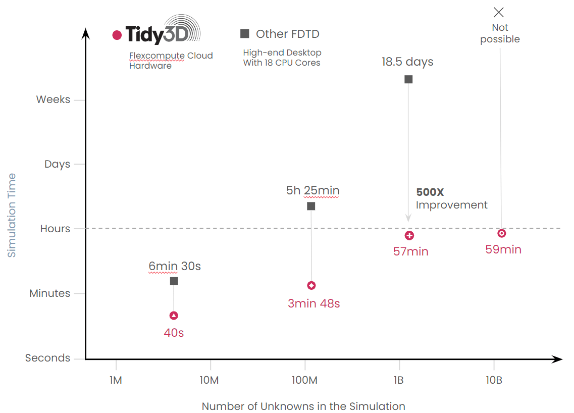
 57min
57min
 59min
59min
What features does the python interface of Tidy3D FDTD provide
Tidy3D contains all of the standard features found in FDTD software, as such it is applicable to almost all problems. For the complete list of Tidy3D Python features and how to use them see the documentation.
A few of the main features include:
Periodic, Bloch periodic, absorbing, and perfect electrically conducting boundary conditions.
May exploit symmetry in the system to speed up simulations by up to 8 times.
Automatic nonuniform meshing, which can auto-generate a discretization scheme for a given geometry to provide finer discretization to regions of the simulation requiring higher accuracy.
Sub-pixel smoothing applied to structure edges, which dramatically improves accuracy for a given simulation discretization setting.
Define device geometry using built in geometric components or GDS and STL file import.
Regular, dispersive, or anisotropic mediums available. And they may also be loaded from an extensive library of materials or fit to experimental data using a built in tool.
Fully featured mode solver for generating modal sources and measuring mode amplitudes, including bent and angled waveguides. Quick set-up of strip, rib, and coupled waveguide geometries.
Several source definitions including plane wave, Gaussian beam, modal source, and user defined current distributions.
Frequency-domain and time-domain monitors for measuring field patterns, flux transmission, and modal amplitudes.
Shape and density-based inverse design framework.
Resonance finder tool to calculate the quality factor of long-lived resonances without the need of running simulations for a long time.
Near field to far field transformation tool for analyzing the far field response of your device without needing to model the entire geometry. May perform server-side computation to save time and reduce data needed to download.
Compatibility between Python UI and GUI
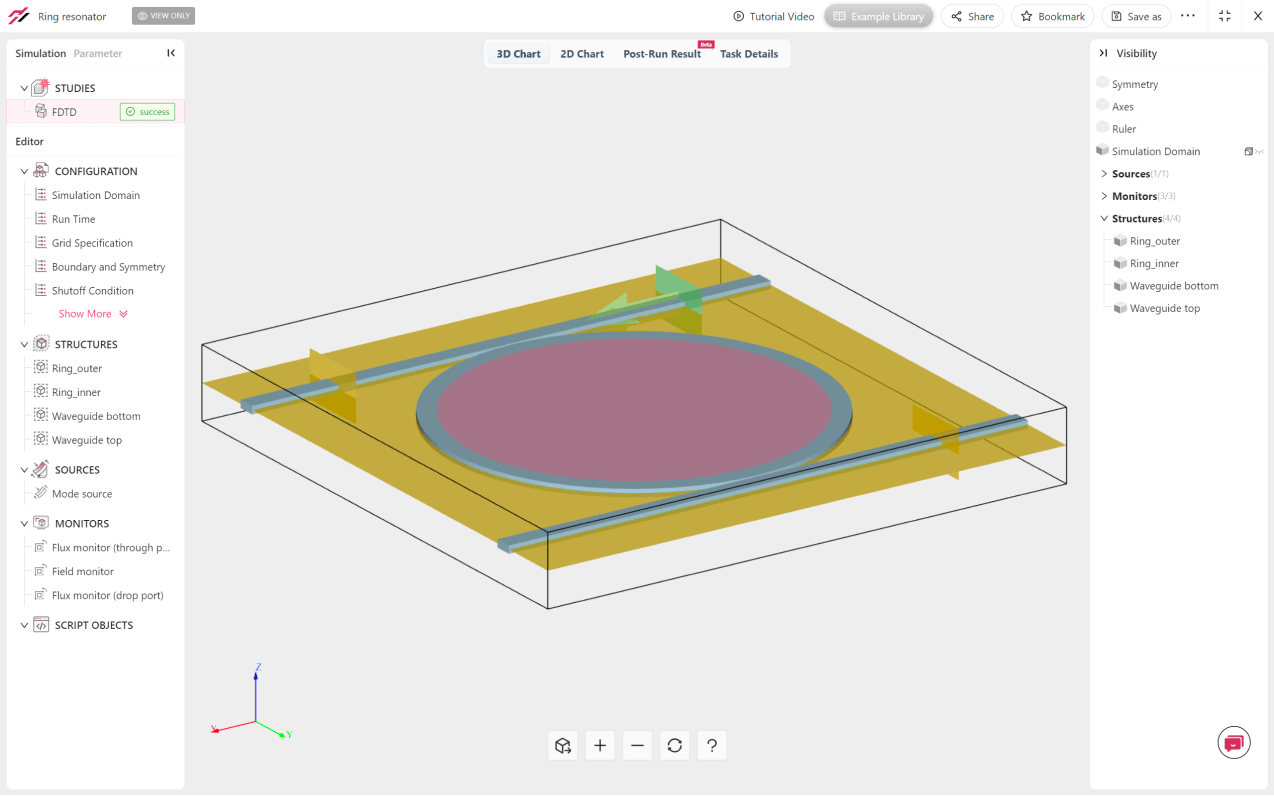
The Tidy3D Python interface generates JSON files containing all the simulation specifications, including structures, sources, and monitor parameters. These files can be opened in the web-based Graphical User Interface (GUI), where all the components can be visualized in a 3D interface. Simulations built using the GUI can also be loaded using Python script.
How is the python interface of Tidy3D FDTD designed
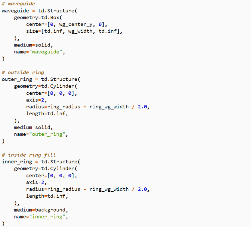
The Tidy3D package allows users to define their simulation programmatically as a collection of basic components, such as geometries, materials, sources, and monitors. Each of these components is a data structure with a well-defined schema combined with validations that ensure that the contents are properly set up. These validations ensure that if a simulation is set up incorrectly, it is immediately caught before starting the FDTD, which saves time and effort. Here is an example
import tidy3d as td
# try to make a box with negative size in one dimension box = td.Box(size=(-1, 1, 1))
"""
1 validation error for Box
size -> 0
   ensure this value is greater than or equal to 0 (type=value_error.number.not_ge; limit_value=0)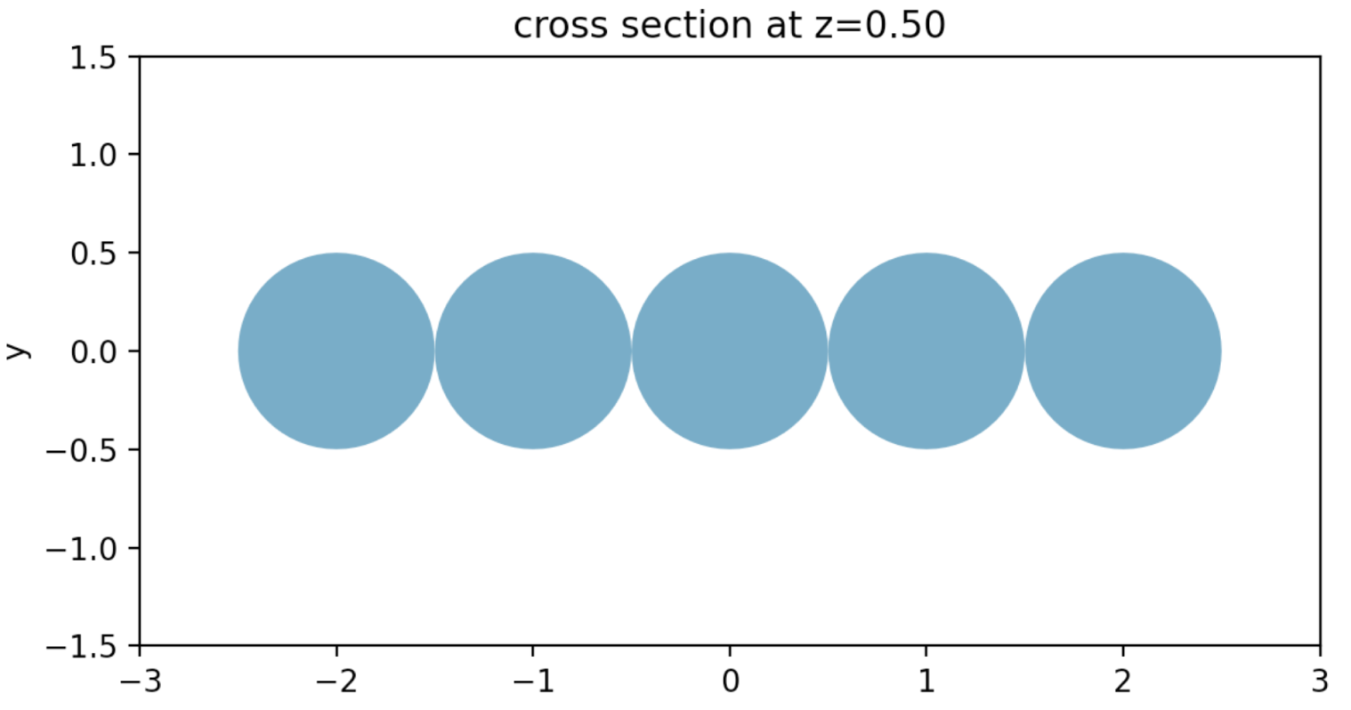
"""All components are combined into a single Simulation object, which defines an FDTD simulation and can be easily visualized, validated, and exported to a JSON file. We leverage the pydantic python package to define these components. Here is a minimum working example of a Simulation object containing 5 cylinders that are defined programmatically by looping over their positions.
import tidy3d as td
# generate 5 dielectric cylinders by looping over some positions
dielectric = td.Medium(permittivity=4.0)
cylinders = []
for position in [-2, -1, 0, 1, 2]:
    cylinder = td.Cylinder(radius=0.5, center=(position, 0, 0), length=10, axis=2)
    structure = td.Structure(geometry=cylinder, medium=dielectric)
    cylinders.append(structure)

point_dipole = td.PointDipole(
    center=(0, 0, 1),
    source_time=td.GaussianPulse(freq0=2e14, fwidth=3e13),
    polarization='Ex',
)

monitor = td.FieldMonitor(
     size=(td.inf, td.inf, 0),
     freqs=[2e14],
     name='field'
)

# combine everything into a single Simulation object
sim = td.Simulation(
    size=(6, 3, 6),
    structures=cylinders,
    sources=[point_dipole],
    monitors=[monitor],
    run_time=1e-12,
)Next, the simulation is sent to Flexcompute’s servers through a simple API call from python. The progress of the job is monitored in real time and other functionalities for controlling the job are available directly from python.
import tidy3d.web as web
sim_data = web.run(sim, task_name='my_simulation')
# while the task is running, the status is monitored. # the results are loaded into the `sim_data` object.Finally, the results are loaded into a SimulationData object, which contains the data for each of the supplied monitors. The data is stored in .hdf5 format and the xarray python package is used to provide a convenient interface for performant plotting, selection, interpolation, and post-processing of the data.
# interpolate the Ex field component at a specific point and frequency
Ex_at_origin = data['field'].Ex.interp(x=0, y=0, z=0, f=2e14)As the simulation times are typically on the order of seconds to minutes, this whole process is seamlessly performed within the same python session or broken into different sessions if desired. If one wants to run several simulations in parallel, there is an interface for batch processing of jobs.
How do we visualize results in python
If we have a working Simulation defined, one easy way to visualize it is through the .plot method, which accepts spatial coordinates. For example, using the simulation defined earlier.
import matplotlib.pylab as plt
ax = sim.plot(z=0)
ax.set_tile('my simulation')
plt.show()gives the following plot.
Data can be plotted in a similar way as the SimulationData object and its contents contain .plot_field() and .plot() methods, respectively. More information on plotting and visualization can be seen in our documentation and in the following examples.
Running FDTD through python or jupyter notebook
Many of the examples in the Tidy3D documentation are written in the form of jupyter notebooks. These notebooks allow users to run code in different sections, which can also contain text or images. It is also a convenient format for sharing code examples or running python through the browser, for example google colab. All of the examples found in our documentation can be downloaded directly as jupyter notebooks from the GitHub repository for the documentation, linked here. A Python notebook environment is also hosted at Tidy3D GUI for your convenience. Tidy3D can be run in notebook format, or regular python script, which may be more convenient for “power users” who may want to create more complex workflows surrounding Tidy3D simulations.
Talk to our Tidy3D experts to get a DemoInstalling python or use web-based python
Tidy3D works on any python version 3.7 or above. As such, it can be run using your local version of python. For more details on setting up python locally, more information can be found here. If one doesn’t want to set up python locally, another alternative is to use a web-based service for running python in the browser, such as google colab or binder. Since the FDTD simulations themselves are run through Flexcompute servers, all of the previous approaches are compatible with the python client, which allows users to initialize simulations and work with their resulting data.
How do I sign up for Tidy3D
Use of Tidy3D requires an account to be able to submit jobs to our sever. You can sign up and try if for FREE.
Sign up for Free
