Author: Amberly Xie, Harvard University
1D photonic crystal cavities enhance light-matter interaction for point defects, improving zero phonon line emission, which is essential for many quantum applications involving solid-state point defects. This notebook contains code for designing 1D photonic crystal cavities in 4H-SiC.
First, we will perform a band structure calculation to examine the photonic band gap. Next, we will simulate the full cavity and use the ResonanceFinder plugin to obtain the resonance frequency and quality factor.
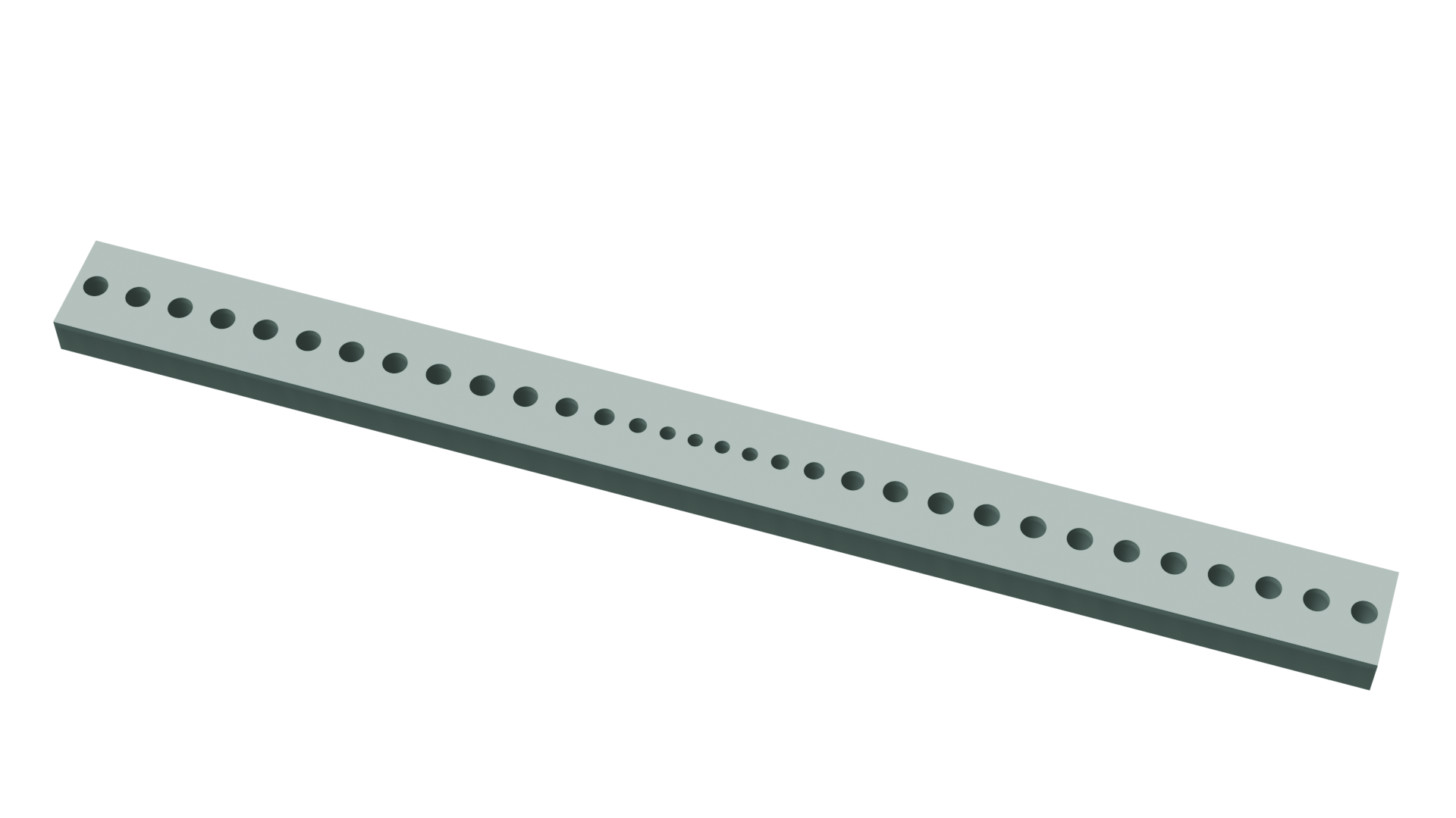
The cavity consists of two stacks of unit cells with the photonic band gap tuned to the desired resonance frequency, and a tapered region where the unit cell parameters are gradually modified to confine the resonance mode.
This notebook is associated with the publication Amberly H. Xie, Aaron M. Day, Jonathan R. Dietz, Chang Jin, Chaoshen Zhang, Eliana Mann, Zhujing Xu, Marko Loncar, and Evelyn L. Hu, Nano Letters 2025 25 (43), 15637-15642. DOI: 10.1021/acs.nanolett.5c04169.
Importing Packages and Defining Useful Functions
import matplotlib.pyplot as plt
import numpy as np
import tidy3d as td
from tidy3d import web
from tidy3d.plugins.resonance import ResonanceFinder
# --- Function for filtering resonances ---
def filter_resonances(resonance_data, minQ, minamp, maxerr):
    resonance_data = resonance_data.where(abs(resonance_data.Q) > minQ, drop=True)
    resonance_data = resonance_data.where(resonance_data.amplitude > minamp, drop=True)
    resonance_data = resonance_data.where(resonance_data.error < maxerr, drop=True)
    resonance_data = resonance_data.where(resonance_data.freq > 0, drop=True)
    return resonance_data
# --- Function to convert from freq to nm ---
def freq_nm(freq):
    return (td.C_0 / freq) * 1e3
# --- Function to find the cavity mode ---
def cavitymode(resonance_data):
    freq = resonance_data.freq
    nm = freq_nm(freq)
    Q = resonance_data.Q
    amplitude = resonance_data.amplitude
    cost = (amplitude * Q) / (np.pi * nm)
    idx = cost.argmax()
    return float(freq[idx]), float(Q[idx])
# --- Function to calculate mode volume ---
def findvmode(sim, data, field_mnt, eps_mnt, freq0):
    # Get grid points
    xaxis = np.array(data[eps_mnt].eps_xx.x)
    yaxis = np.array(data[eps_mnt].eps_xx.y)
    zaxis = np.array(data[eps_mnt].eps_xx.z)

    # Get E-field data
    Ex = np.array(data[field_mnt].Ex).squeeze()
    Ey = np.array(data[field_mnt].Ey).squeeze()
    Ez = np.array(data[field_mnt].Ez).squeeze()
    E_sqr = np.abs(Ex) ** 2 + np.abs(Ey) ** 2 + np.abs(Ez) ** 2
    E_sqr_pad = np.pad(E_sqr, ((0, 1), (0, 1), (0, 1)), "constant")
    eps = (np.array(data[eps_mnt].eps_xx).squeeze()).real

    # Calculate mode volume
    vmode = (
        np.trapz(
            np.trapz(np.trapz(eps * E_sqr_pad, xaxis, axis=0), yaxis, axis=0),
            zaxis,
            axis=0,
        )
    ) / (np.max(eps * E_sqr_pad))
    n_sic = 2.59

    # Normalize mode volume
    wv = freq_nm(freq0) * 1e-3
    vmode = vmode / ((wv / n_sic) ** 3)

    return vmode
Simulating Mirror Cells
We begin by simulating the band structure for the mirror cells, targeting a bandgap centered around surface state emission (700nm).
# --- Simulation parameters ---
epAir = 1
epSic = 2.6**2

# Frequency range of interest
ss1 = td.C_0 / (400e-3)
ss2 = td.C_0 / (1000e-3)
ss0 = td.C_0 / (700e-3)
ssWidth = 149999999997498 / 2.35

# Runtime
runtime = 800 / ssWidth
tstart = 5 / ssWidth
Building the Simulation
# --- Function for creating ellipse unit cells ---
def ellipse_uc(center, x_axis, y_axis, height=0.5):
    theta = np.linspace(0, np.pi * 2, 1001)
    x = x_axis * np.cos(theta) + center[0]
    y = y_axis * np.sin(theta) + center[1]

    geometry = td.PolySlab(
        vertices=np.array([x, y]).T,
        slab_bounds=(-height / 2 + center[2], height / 2 + center[2]),
        axis=2,
    )
    return geometry
# --- Setting up simulation ---
def makecells(params):
    a = params[0]  # Lattice constant
    a1 = params[1]  # X width of holes
    a2 = params[2]  # Y width of holes
    w = params[3]  # Width of beam
    h = 0.3  # Thickness

    matSlab = td.Medium(permittivity=epSic, name="matSlab")
    matHole = td.Medium(permittivity=epAir, name="matHole")

    slab = td.Structure(
        geometry=td.Box(
            center=(0, 0, 0),
            size=(td.inf, w, h),
        ),
        medium=matSlab,
        name="slab",
    )

    hole = td.Structure(
        geometry=ellipse_uc((0, 0, 0), a1, a2, height=0.5), medium=matHole, name="hole"
    )

    structures = [slab, hole]

    # Sources and monitors

    numDipoles = 5
    numMonitors = 2

    polarization = "Ey"

    rng = np.random.default_rng(12345)
    dipolePos = rng.uniform([-a / 2, -w / 2, 0], [a / 2, w / 2, 0], [numDipoles, 3])
    monitorPos = rng.uniform([-a / 2, -w / 2, 0], [a / 2, w / 2, 0], [numDipoles, 3])

    dipolePhase = rng.uniform(0, 2 * np.pi, numDipoles)

    pulses = []
    dipoles = []
    for i in range(numDipoles):
        pulse = td.GaussianPulse(freq0=ss0, fwidth=ssWidth, phase=dipolePhase[i])
        pulses.append(pulse)
        dipoles.append(
            td.PointDipole(
                source_time=pulse,
                center=tuple(dipolePos[i]),
                polarization=polarization,
                name="dipole-" + str(i),
            )
        )

    monitorsTime = []
    for i in range(numMonitors):
        monitorsTime.append(
            td.FieldTimeMonitor(
                fields=["Ey"],
                center=tuple(monitorPos[i]),
                size=(0, 0, 0),
                start=tstart,
                name="monitor-time-" + str(i),
            )
        )

    # Boundary conditions

    bspecs = td.BoundarySpec(
        x=td.Boundary.bloch(0.5), y=td.Boundary.pml(), z=td.Boundary.pml()
    )

    simSize = (a, 2, 4)

    return [structures, dipoles, monitorsTime, simSize, bspecs]
Running the Simulation
params = [0.198, 0.066, 0.066, 0.345]
structures = makecells(params)[0]
dipoles = makecells(params)[1]
monitorsTime = makecells(params)[2]
simSize = makecells(params)[3]
bspecs = makecells(params)[4]
symmetry = (0, 0, 1)
sim = td.Simulation(
center=(0, 0, 0),
size=simSize,
grid_spec=td.GridSpec.auto(),
structures=structures,
sources=dipoles,
monitors=monitorsTime,
run_time=runtime,
shutoff=0,
boundary_spec=bspecs,
normalize_index=None,
symmetry=symmetry,
)
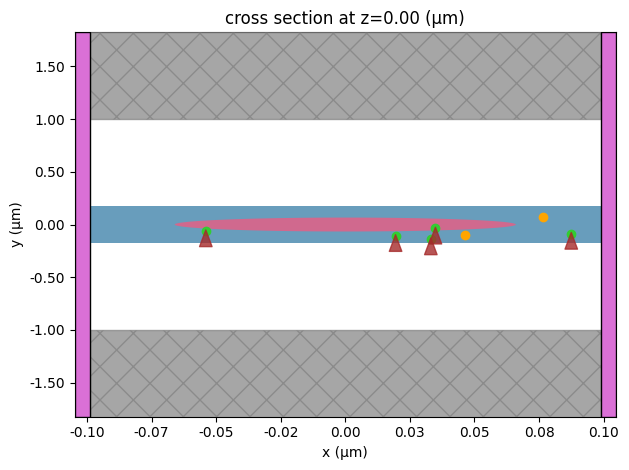
ax = sim.plot(z=0)
ax.set_ylim(-0.5, 0.5)
plt.show()
# Upload task
task_id = web.upload(sim, task_name="NBBands")
# Run simulation
NBBandsData = web.run(
    sim, "NBBands", folder_name="data", path="data/NBBands.hdf5", verbose=True
)
15:26:14 -03 Created task 'NBBands' with task_id
             'fdve-bc57a594-ed6c-43a3-8600-342ba02c6374' and task_type 'FDTD'.
             View task using web UI at
             'https://tidy3d.simulation.cloud/workbench?taskId=fdve-bc57a594-ed6
             c-43a3-8600-342ba02c6374'.
Task folder: 'default'.
Output()
15:26:17 -03 Maximum FlexCredit cost: 0.025. Minimum cost depends on task
             execution details. Use 'web.real_cost(task_id)' to get the billed
             FlexCredit cost after a simulation run.
15:26:18 -03 Created task 'NBBands' with task_id
             'fdve-607246f3-115c-43e2-afe7-7a4ab07811e5' and task_type 'FDTD'.
             View task using web UI at
             'https://tidy3d.simulation.cloud/workbench?taskId=fdve-607246f3-115
             c-43e2-afe7-7a4ab07811e5'.
Task folder: 'data'.
Output()
15:26:20 -03 Maximum FlexCredit cost: 0.025. Minimum cost depends on task
             execution details. Use 'web.real_cost(task_id)' to get the billed
             FlexCredit cost after a simulation run.
15:26:22 -03 status = success
Output()
15:26:28 -03 loading simulation from data/NBBands.hdf5
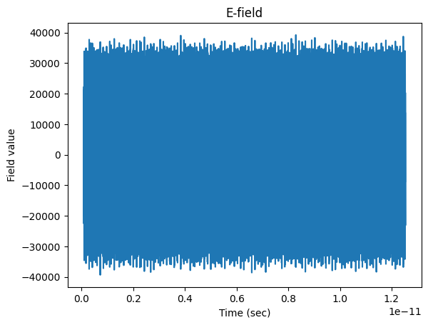
# Plotting E field as a function of time
plt.plot(
NBBandsData.monitor_data["monitor-time-0"].Ey.t,
np.real(NBBandsData.monitor_data["monitor-time-0"].Ey.squeeze()),
)
plt.xlabel("Time (sec)")
plt.ylabel("Field value")
plt.title("E-field")
plt.show()
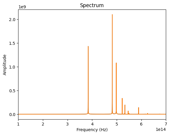
# Plot spectra
time_series = np.real(NBBandsData.monitor_data["monitor-time-0"].Ey.squeeze())
dt = NBBandsData.simulation.dt
fmesh = np.fft.fftshift(np.fft.fftfreq(time_series.size, dt))
spectrum = np.fft.fftshift(np.fft.fft(time_series))
plt.plot(fmesh, np.abs(spectrum))
time_series = np.real(NBBandsData.monitor_data["monitor-time-0"].Ey.squeeze())
dt = NBBandsData.simulation.dt
fmesh = np.fft.fftshift(np.fft.fftfreq(time_series.size, dt))
spectrum = np.fft.fftshift(np.fft.fft(time_series))
plt.plot(fmesh, np.abs(spectrum))
plt.xlim(1e14, 7e14)
plt.title("Spectrum")
plt.xlabel("Frequency (Hz)")
plt.ylabel("Amplitude")
plt.show()
# Run resonance finder
resonance_finder = ResonanceFinder(freq_window=tuple((ss2, ss1)))
resonance_data = resonance_finder.run(signals=NBBandsData.data)
# Filter resonances
resonance_data_filtered = filter_resonances(
resonance_data=resonance_data, minQ=100, minamp=0.001, maxerr=100
)
freqs = resonance_data_filtered.freq.to_numpy()
# Target frequency
v0 = 428274940000000
# Center frequency
v1 = None
v2 = None
for freq in freqs:
if freq < v0:
v1 = freq
elif freq > v0:
v2 = freq
break
# Calculating band edges
print(f"Wavelength 1: {freq_nm(v1):.2f}")
print(f"Wavelength 2: {freq_nm(v2):.2f}")
Wavelength 1: 780.02
Wavelength 2: 621.99
Simulating 1D Photonic Crystal Cavity
Building the Simulation
# --- Set up structures ---
def makecells(params):
    a = params[0]  # Lattice constant
    a1 = params[1]  # X width
    a2 = params[2]  # Y width
    w = params[3]  # Width of beam
    t = params[4]  # Taper constant
    nummirr = 12  # Number of mirror cells on each side
    numtaper = 8  # Half the number of taper cells
    h = 0.3  # Thickness

    matSlab = td.Medium(permittivity=epSic, name="matSlab")
    matHole = td.Medium(permittivity=epAir, name="matHole")

    # Array to hold lattice constants
    latticeconsttemp = []
    a1temp = []
    a2temp = []

    # Adding mirror cell lattice constants
    for i in np.arange(0, nummirr):
        latticeconsttemp.append(a)
        a1temp.append(a1)
        a2temp.append(a2)

    # Adding taper cell lattice constants
    for i, num in enumerate(np.arange(0, numtaper)):
        latticeconsttemp.append((t ** (i + 1)) * a)
        a1temp.append((t ** (i + 1)) * a1)
        a2temp.append((t ** (i + 1)) * a2)

    latticeconstL = latticeconsttemp
    latticeconstR = latticeconsttemp[::-1]
    a1L = a1temp
    a1R = a1temp[::-1]
    a2L = a2temp
    a2R = a2temp[::-1]

    structures = []

    slab = td.Structure(
        geometry=td.Box(
            center=(0, 0, 0),
            size=(td.inf, w, h),
        ),
        medium=matSlab,
        name="slab",
    )

    structures.append(slab)

    # Setting up nanobeam
    for i, const in enumerate(latticeconstL):
        center = (-np.sum(latticeconstL[i + 1 :]) - const / 2, 0, 0)
        hole = td.Structure(
            geometry=ellipse_uc(center, a1L[i], a2L[i], height=0.5),
            medium=matHole,
            name="holeL" + str(i),
        )

        structures.append(hole)

    for i, const in enumerate(latticeconstR):
        center = (np.sum(latticeconstR[:i]) + const / 2, 0, 0)
        hole = td.Structure(
            geometry=ellipse_uc(center, a1R[i], a2R[i], height=0.5),
            medium=matHole,
            name="holeR" + str(i),
        )

        structures.append(hole)

    # Set up sources and monitors

    source = td.PointDipole(
        center=(0, 0, 0),
        source_time=td.GaussianPulse(freq0=ss0, fwidth=ssWidth),
        polarization="Ey",
    )

    point_t_mnt = td.FieldTimeMonitor(
        center=[0, 0, 0],
        size=[0, 0, 0],
        start=tstart,
        name="point",
        colocate=True,  # Colocate so field is colocated to grid cell centers
    )

    field_t_mnt = td.FieldTimeMonitor(
        center=[0, 0, 0],
        size=[td.inf, td.inf, td.inf],
        start=runtime,
        name="field",
        colocate=True,
    )

    eps_mnt = td.PermittivityMonitor(
        center=[0, 0, 0], size=[td.inf, td.inf, td.inf], freqs=[ss0], name="eps"
    )

    # Boundary conditions
    bspecs = td.BoundarySpec(
        x=td.Boundary.pml(), y=td.Boundary.pml(), z=td.Boundary.pml()
    )

    simSize = (a * 2 * len(latticeconstL) * 1.1, w * 5, 1.5)

    return structures, simSize, bspecs, source, point_t_mnt, field_t_mnt, eps_mnt
Running the simulation
params = [0.198, 0.066, 0.066, 0.345, 0.97]

simsetup = makecells(params)

structures = simsetup[0]
simSize = simsetup[1]
bspecs = simsetup[2]
source = simsetup[3]
point_t_mnt = simsetup[4]
field_t_mnt = simsetup[5]
eps_mnt = simsetup[6]
symmetry = (1, -1, 1)

mesh_override = td.MeshOverrideStructure(
    geometry=td.Box(center=(0, 0, 0), size=(0.5, 0.5, 0.5 * 1.5)), dl=[0.01, 0.01, 0.01]
)

# Define grid specification for the simulation
grid_spec = td.GridSpec.auto(
    min_steps_per_wvl=10,
    override_structures=[mesh_override],
)


sim = td.Simulation(
    center=(0, 0, 0),
    size=simSize,
    grid_spec=td.GridSpec.auto(),
    structures=structures,
    sources=[source],
    monitors=[point_t_mnt, field_t_mnt, eps_mnt],
    run_time=runtime,
    shutoff=0,
    boundary_spec=bspecs,
    normalize_index=None,
    symmetry=symmetry,
)

sim.plot(z=0)
plt.show()
# Upload task
task_id = web.upload(sim, task_name="NBSym")
# Run simulation
NBSymData = web.run(
    sim, "NBSym", folder_name="data", path="data/NBSym.hdf5", verbose=True
)
15:26:36 -03 Created task 'NBSym' with task_id
             'fdve-1db7c742-a4c9-4f6c-9fe7-632e467dabf5' and task_type 'FDTD'.
             View task using web UI at
             'https://tidy3d.simulation.cloud/workbench?taskId=fdve-1db7c742-a4c
             9-4f6c-9fe7-632e467dabf5'.
Task folder: 'default'.
Output()
15:26:41 -03 Maximum FlexCredit cost: 0.039. Minimum cost depends on task
             execution details. Use 'web.real_cost(task_id)' to get the billed
             FlexCredit cost after a simulation run.
             Created task 'NBSym' with task_id
             'fdve-8e295aef-41f2-4968-b8cf-c00df61e8adf' and task_type 'FDTD'.
             View task using web UI at
             'https://tidy3d.simulation.cloud/workbench?taskId=fdve-8e295aef-41f
             2-4968-b8cf-c00df61e8adf'.
Task folder: 'data'.
Output()
15:26:46 -03 Maximum FlexCredit cost: 0.039. Minimum cost depends on task
             execution details. Use 'web.real_cost(task_id)' to get the billed
             FlexCredit cost after a simulation run.
15:26:47 -03 status = success
Output()
15:27:03 -03 loading simulation from data/NBSym.hdf5
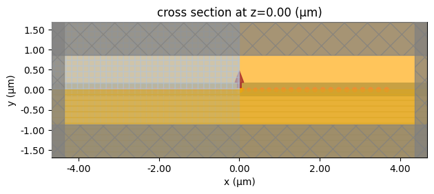
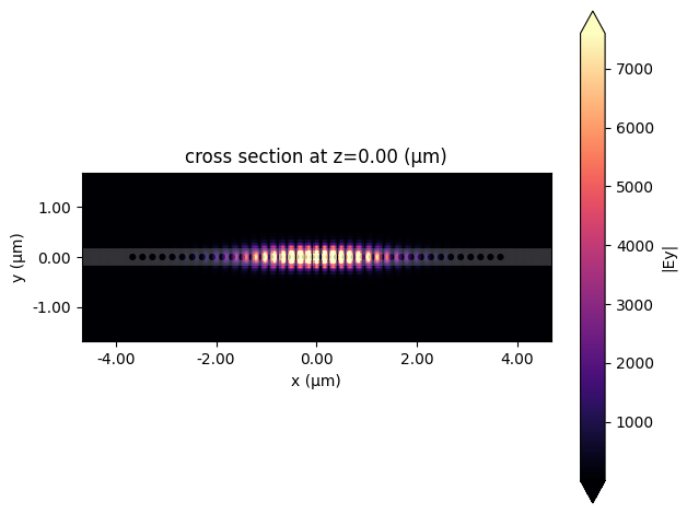
# Plotting E field at very end of simulation
final_time = NBSymData["field"].Ey.t
NBSymData.plot_field("field", "Ey", val="abs", t=final_time, z=0)

plt.show()
# Get y-component of E field from point monitor
time_series = NBSymData["point"].Ey.squeeze()

# Run resonance finder
resonance_finder = ResonanceFinder(freq_window=tuple((ss2, ss1)))
resonance_data = resonance_finder.run_scalar_field_time(time_series)
resonance_data_filtered = filter_resonances(
    resonance_data=resonance_data, minQ=100, minamp=0.001, maxerr=100
)

# Cavity mode with highest Q from filtered resonances
freqcav, Q = cavitymode(resonance_data_filtered)

print(f"Resonance frequency: {freq_nm(freqcav):.2f} nm")
print(f"Quality Factor: {Q}")
Resonance frequency: 691.01 nm
Quality Factor: 1997968.1586556784
Notes on Q-factor calculations
In this example, a relatively broadband excitation was used. This method is useful when the exact resonance frequency is not known beforehand, but it can also excite modes other than the fundamental one, which increases the error in the Q-factor calculation.
For a more precise Q-factor calculation, a second simulation with a narrow band around the resonance can be used.