Plasmonic nanoparticles can exhibit interesting electromagnetic properties at certain frequencies, such as a negative real part of the relative permittivity. Due to their high electrical conductivity, gold nanoparticles can be challenging to model: the rapid field variations inside and near the particles require a fine local discretization. Therefore, an intelligent non-uniform meshing scheme is essential to make sure that the particle is well resolved, while ensuring that the empty space around it does not lead to wasted simulation effort.

Scattering from a 10 nm gold sphere is modeled in this example, and results are compared to the analytical Mie series. This example uses the total-field-scattered-field (TFSF) source to excite the particle, and illustrates how to compute various quantities like the total absorbed power, total scattering cross-section, and forward cross-section. A non-uniform mesh is carefully designed to make sure the sphere is well resolved without a significant sacrifice in efficiency. For a more detailed demonstration on TFSF, please refer to the TFSF tutorial.

For more simulation examples, please visit our examples page. If you are new to the finite-difference time-domain (FDTD) method, we highly recommend going through our FDTD101 tutorials. FDTD simulations can diverge due to various reasons. If you run into any simulation divergence issues, please follow the steps outlined in our troubleshooting guide to resolve it.

Define the structure and boundary conditions¶

Note the special treatment in creating the mesh: we need to make sure that the mesh is sufficiently fine within the sphere, but we can also make use of Tidy3D's non-uniform meshing algorithm to have a coarser grid outside the sphere, for better efficiency. Furthermore, the TFSF source works best if placed in a region with uniform mesh. Because of this, we will add a mesh override structure which is slightly larger than the sphere itself.

Create Source¶

For our incident field, we use a TFSF source to inject a plane wave incident from below the sphere polarized in the x direction.

Create Monitors¶

Next, we define a number of monitors to analyze the simulation.

• A 3D FluxMonitor inside the TFSF source can be used to compute the power absorbed in the particle. If no power is absorbed, the recorded flux would be 0, since there are no power sources or sinks inside the monitor box. Any flux recorded in the FluxMonitor is then due to the imbalance between the incoming power and the outgoing one, which has been reduced by the particle absorption.

• A 3D FluxMonitor outside the TFSF region can be used to compute the total cross-section, meaning the total power of scattered radiation in all directions.

• A FieldProjectionAngleMonitor can be used to compute the radiated cross-section at a particular angle.

• A 3D Field monitor inside the TFSF region to record the electric field is required to compute the absorbed power. The parameter colocate is set to False in order to match with the grid specification of the permittivity monitor.

• A 3D permittivity monitor inside the the TFSF region is required to compute the displacement field $D=\epsilon E$ and the absorbed power. In default settings, colocate is set to False so that the permittivity at the Yee grid locations, exactly as used in the solver, is stored.

• Finally, we also store the fields in a planar cross-section for visualization purposes.

Create Simulation¶

Now we can put everything together and define the simulation.

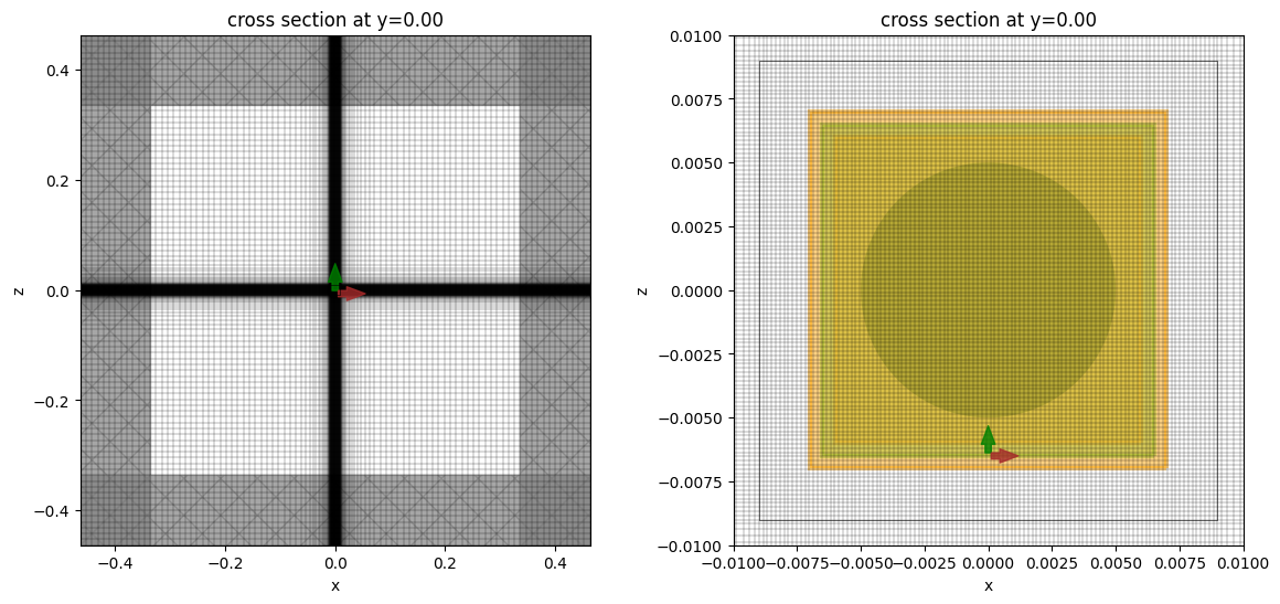
Visualize Geometry and Mesh¶

Let's take a look at the mesh and geometry and make sure everything is defined properly in the simulation. The nanoparticle is very small compared to the simulation and is not visible in the full plot. For better visibility, we also show a zoomed-in plot, which shows how the nanoparticle is meshed. Note that the mesh inside the nanoparticle is quite fine and may not render correctly in the notebook, possibly giving the false impression of being somewhat coarse.

Run Simulation¶

Extract the results¶

Absorbed Power Distribution¶

The dissipated power in a lossy material when subjected to a time-harmonic electromagnetic field is a quantity that can be computed from the electric field $E$ and the permittivity $\varepsilon$. For futher thoretical details, refer to [1].

The volumetric power absorption density, denoted as $p_{\text{abs}}(x, y, z)$, measures the power absorbed per unit volume at a specific point. Realistic metallic properties are described through a complex permittivity $\varepsilon_c = \varepsilon' - j\varepsilon''$. Here, $\varepsilon''$, the imaginary part, accounts for dielectric losses. The volumetric absorption density can be defined as $p_{\text{abs}}(x, y, z) = -\frac{1}{2}\omega\varepsilon''|E|^2$.

A more general way to express this quantity is by using the dot product of the electric $E$ and displacement fields $D$. For a linear isotropic material, given the relation $D = \varepsilon_c E = (\varepsilon' - j\varepsilon'')E$, it is easily verifiable that $\varepsilon'' |E|^2 = -\text{Imag}\{ E^* \cdot D\}$. Substituting this into our derived formula gives $$p_{\text{abs}}(x,y,z) = \frac{1}{2}\omega \text{Imag}\{E^*(x, y, z) \cdot D(x, y, z)\}$$ where:

• $\omega$ is the angular frequency ($2\pi f$) of the field in rad/s.
• $E^*(x, y, z)$ is the complex conjugate of the electric field.
• $D(x, y, z)$ is the electric displacement field.
• $\text{Imag}$ denotes the imaginary part of the argument.

This expression, employing $E^*$ and $D$, is the most general form for losses because it derives directly from Poynting's theorem on energy conservation. It remains universally valid for anisotropic and nonlinear media by using the material's true response $D$, without assuming it must be parallel or proportional to the driving field $E$. To find the total absorbed power ($P_{\text{abs}}$) within a specific volume $V$, one must integrate the volumetric power density over that volume:

$$P_\text{abs} = \int_V p_\text{abs} (x, y, z) = \int_V \frac{1}{2} \omega \; \text{Imag} (E^*(x,y,z) \cdot D (x, y, z))\; dV$$

Using the relation $\omega = 2 \pi f$, this can also be written as:

$$P_\text{abs} = \int_V \pi f \; \text{Imag} (E^*(x,y,z) \cdot D (x, y, z)) \; dV$$

[1] Jian-Ming Jin, Theory and computation of electromagnetic fields sec. 1.7.

The displacement field $D$ can be computed as $D = \epsilon E$. This is possible since colocate=False was set on the electric field monitor, allowing the permittivity and electric field data to be defined with the same grid specifications.

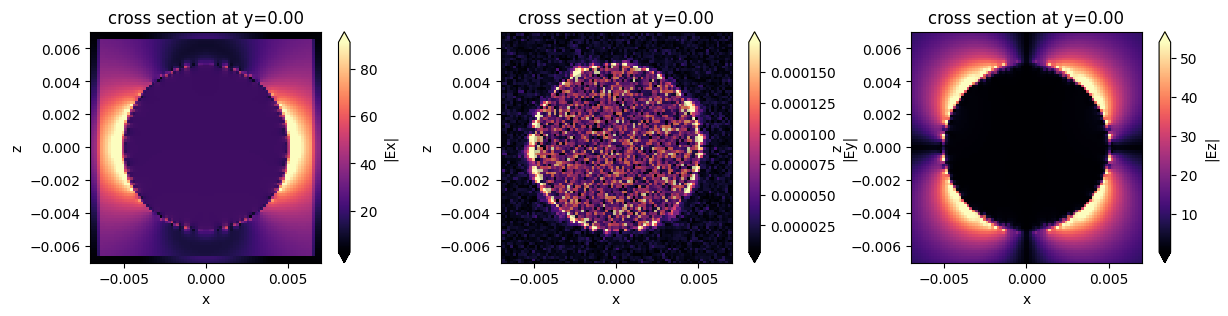
Plot the electric field¶

Plot the absorbed power density¶

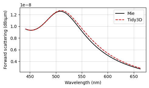
Comparison with Mie Series¶

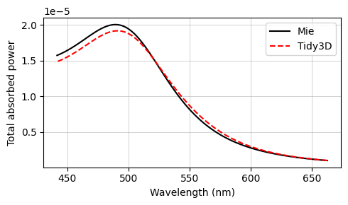
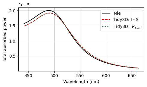
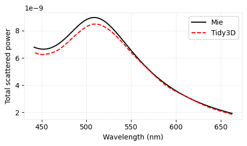
The final results are compared against the analytical Mie series below, and very good agreement is observed. The small deviations can be reduced with a further refinement of the grid. Since the sphere's material is metallic, no subpixel averaging scheme is applied, so the simulation approximates the curved permittivity profile in a staircase-like manner, which contributes to the error. The label Tidy3D: I - S, standing for incoming minus scattered power, denotes the amount of power that is absorbed in the source region measured by calculating the flux flowing inward inside the TFSF region.

The txt files containing the Mie results can be downloaded from our documentation repo.