Hovering Rotor CFD with Flow360 (Part 2 of 3)
In this series of articles, we highlight our efforts to accurately model the flow physics of a hovering helicopter rotor in isolation and installed on a fuselage using the solver Flow360. In Part I, the motivation for the simulations is discussed. Part II provides details on the computational setup, including the rotor blade geometry, the Flow360 CFD solver, the treatment of turbulence, the computational grid, and the sliding interface methodology. Part III presents the simulation results, including the effect of mesh refinement and time resolution, collective sweep studies, and comparisons with experimental data and other CFD codes.
In this 2nd part of the series, we present important details about the geometry of the rotor blades, the simulation grid, and the computational methods we used to model the hovering helicopter rotor.
Flow360 CFD Solver
Our simulation software, Flow360, is based on hardware/software co-design with emerging hardware computing leading to unprecedented solver speed without sacrificing accuracy. The Flow360 solver is a node-centered unstructured grid solver based on a 2nd order finite volume method. The convective fluxes are discretized using the Roe Riemann solver, whereas central differences are used for the viscous fluxes. MUSCL extrapolation is used to achieve higher order accuracy in space. Flow360 includes a number of standard turbulence models including SA-neg, SA-RC, 𝑘 − 𝜔 SST, and DDES. Transition modeling capabilities are also available based on the 3-equation SA-AFT model, but are not used in the present work. All simulations are performed as time-accurate using the dual time-stepping technique with the time derivative discretized using an implicit second-order accurate backward Euler scheme.
Geometry of the HVAB rotor blade
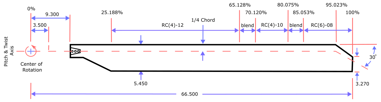
We focus on the 4-bladed HVAB rotor, which is the main topic of the Hover Prediction Workshop. We used the IGS file available on the hover prediction workshop file share site as the baseline blade geometry. As shown in Figure 1, the blade geometry is highly similar to the PSP rotor blade and features a planform with 14 degrees linear twist, RC-series airfoils and a swept-tapered tip (30 degrees sweep, 0.6 taper ratio outboard of 0.95 radius). The radius of the blade is 66.5 inches with a reference chord of 5.45 inches giving a rotor solidity of 0.1033. The flap hinge is located at 3.5 inches from the rotor axis with the lag hinge assumed to be coincident.
Fuselage
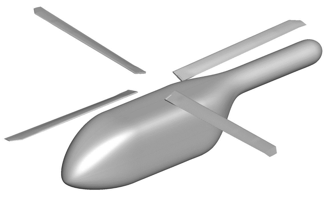
For installed rotor calculations, the NASA Robin-mod7 fuselage is used as recommended by the hover focus problem. This generic fuselage has an analytical definition with the cross sections defined by a series of superellipses. The fuselage geometry was generated in Engineering Sketch Pad (ESP) using 45 cross sections and compared visually to the Plot3D geometry available on the hover prediction workshop file share site. The geometry does not include the main rotor pylon or the rotor hub. The fuselage has a length of 123.931 inches and was pitched up by 3.5 degrees. The full configuration of the HVAB blades with the fuselage is shown in Figure 2.
Sliding Interface Methodology
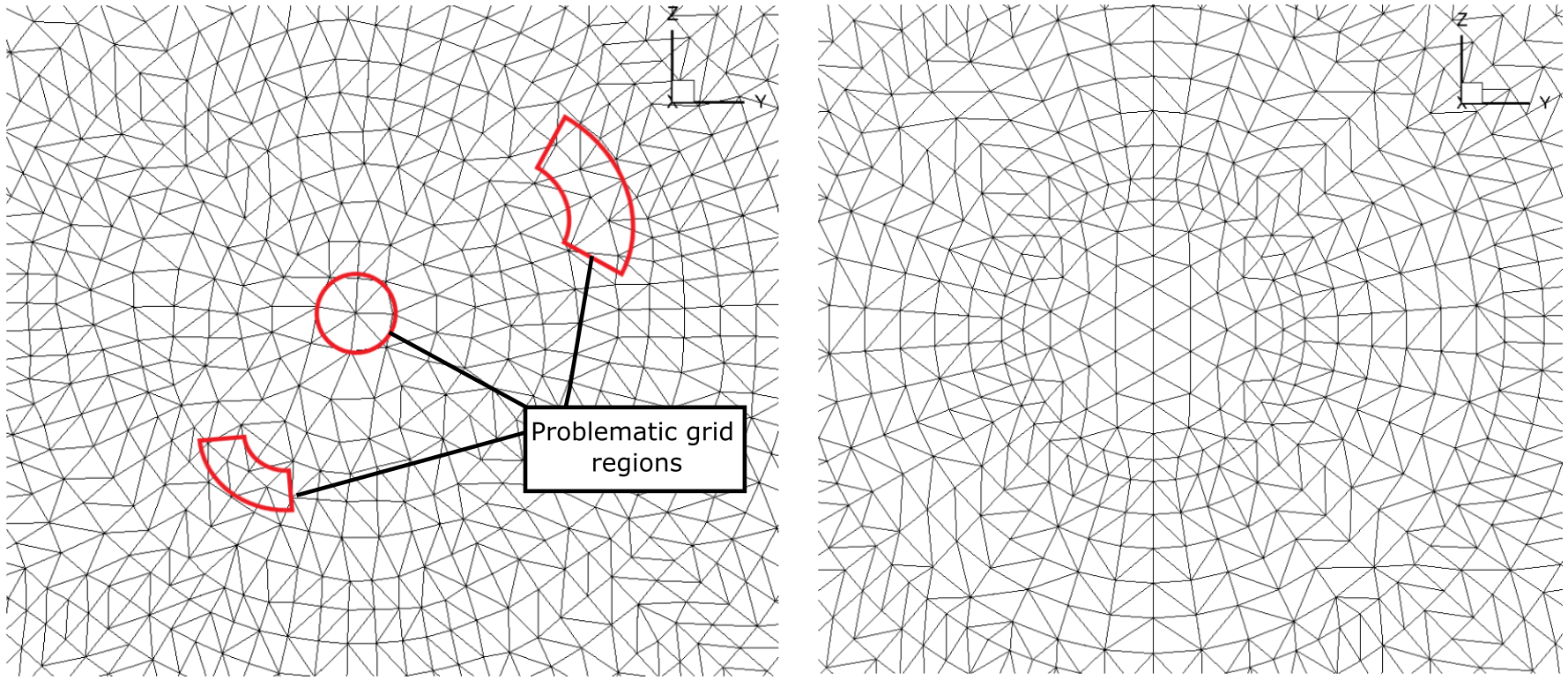
In order to efficiently simulate rotating blades, Flow360 solver uses the sliding interface methodology to model the relative motion of individual components. The domain is split into a nearfield rotating block which encloses the rotor blades and a farfield stationary block which contains the fuselage in the case of installed rotor cases. The blocks do not overlap. Data is interpolated between the two blocks in the y-z plane using a 2nd order scheme. To minimize the computational costs, strict constraints are imposed on the node layout on the sliding interface, as all nodes must lie on concentric circles, as shown in Figure 3. This leads to a significant reduction in computational overhead as no interpolation weights need to be calculated or stored as the position of each node is known at every time step.
As the rotor was modeled using a sliding interface method for rotation, the meshes had to be regenerated for each collective angle and mesh refinement level. This was done by imposing the pitch, flap, and lag angles on the geometry through a series of translations and rotations.
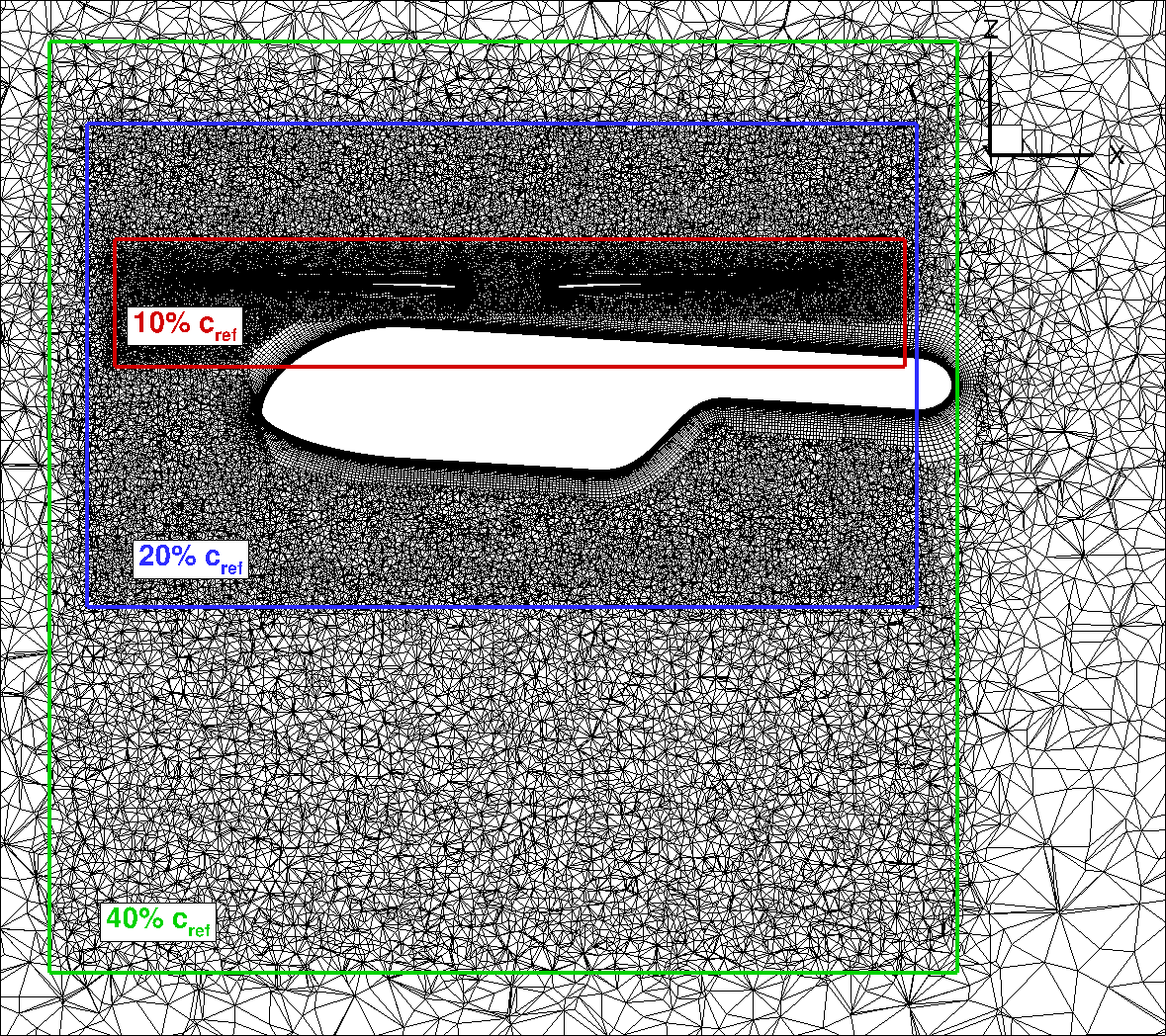
To study the effect of mesh resolution, five mesh levels were generated and their resolution expressed in terms of the reference chord length (cref) of 5.45 inches. The values used were 20% cref, 15% cref, 10% cref, 7.5% cref (see Fig. 4), and 5% cref. For the surface mesh, the maximum edge length was set to 0.545 for the 10% cref mesh, and the refinement factor value was used to generate the other meshes. The curvature resolution parameter was set to 5 degrees to control the resolution at the leading edge, trailing edge, and blade tip.
The volume mesh used for this analysis is split into a rotating nearfield block and a farfield stationary block. The sliding interface is placed between -0.075R and 0.105R to allow anisotropic layers to grow on the fuselage surface. Wall-normal spacing is set to ensure 𝑦+<1 on the surfaces. The mesh uses hexahedral elements in the blade boundary layers and prism elements in the fuselage boundary layer, which transition to a tetrahedral mesh in the farfield. Three levels of refinement are used to resolve the wake.
The flow in the simulation is first initialized using a 1st order solver for one revolution with a 6 degree time step, followed by 18 to 24 revolutions computed using a 2nd order solver using the same time step to establish the wake and advect the starting vortex. The simulation is continued using lower time steps, with error bars included in the integrated load results to account for long transients and low sample size. The blade was modeled as rigid, and the SA-RC-DDES turbulence model was used. The final loading results are averaged over 5 revolutions, and the confidence interval is of the same order of magnitude as the standard deviation due to the low sample size.
This concludes Part II of the series. In the next article we will discuss the results we obtained in the study and discuss their implications.
If you’d like to learn more about CFD simulations, how to optimize them, or how to reduce your simulation time from weeks or days to hours or minutes, stop by our website at flexcompute.com or follow us on LinkedIn.
For the expanded version of the paper this content is derived from, click here.