Hovering Rotor CFD with Flow360 (Part 3 of 3)
In this series of articles, we highlight our efforts to accurately model the flow physics of a hovering helicopter rotor in isolation and installed on a fuselage using the solver Flow360. In Part I, the motivation for the simulations was discussed. Part II provided details on the computational setup, including the rotor blade geometry, the Flow360 CFD solver, the treatment of turbulence, the computational grid, and the sliding interface methodology. Part III presents the simulation results, including the effect of mesh refinement and time resolution, collective sweep studies, and comparisons with experimental data and other CFD codes.
In this 3rd and last part of the series, we present the results we obtained by simulating a hovering rotor using our solver Flow360.
Definitions
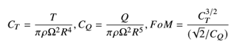
Before presenting the results, let us first define the integrated loads and sectional loads. The thrust coefficient, torque coefficient and figure of merit (FoM) are defined as follows:
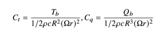
The sectional loads are normalized by the local chord and the local velocity as follows:
Isolated Rotor Setup
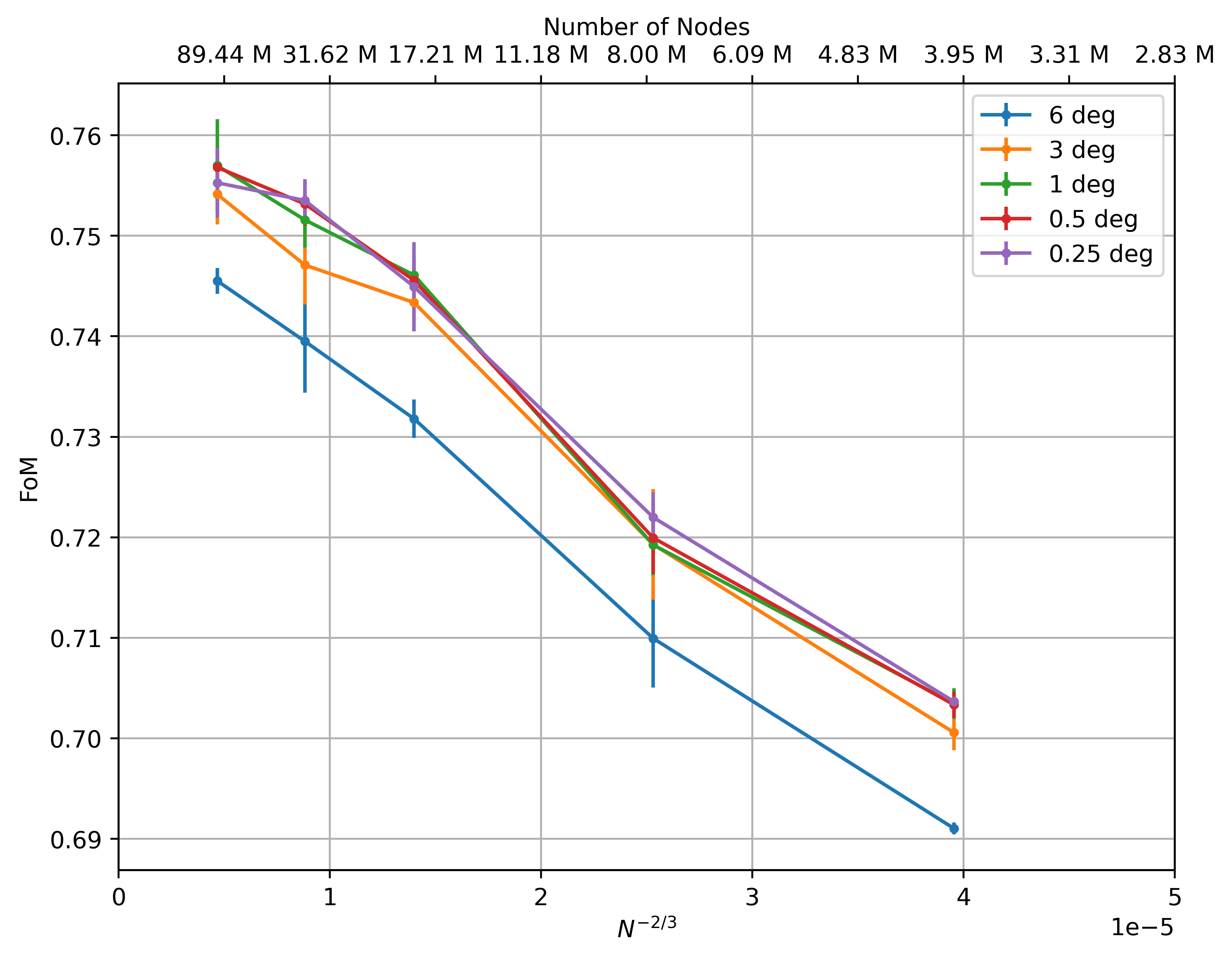
The integrated loads convergence for the isolated rotor with a mesh refinement and time step is shown in Figure 1. The FoM calculated from the integrated loads is plotted versus grid factor for different time steps, where N is the number of mesh nodes for the mesh refinement study. The power -⅔ for N would give straight lines with ideal 2nd-order convergence and in a family of grids.
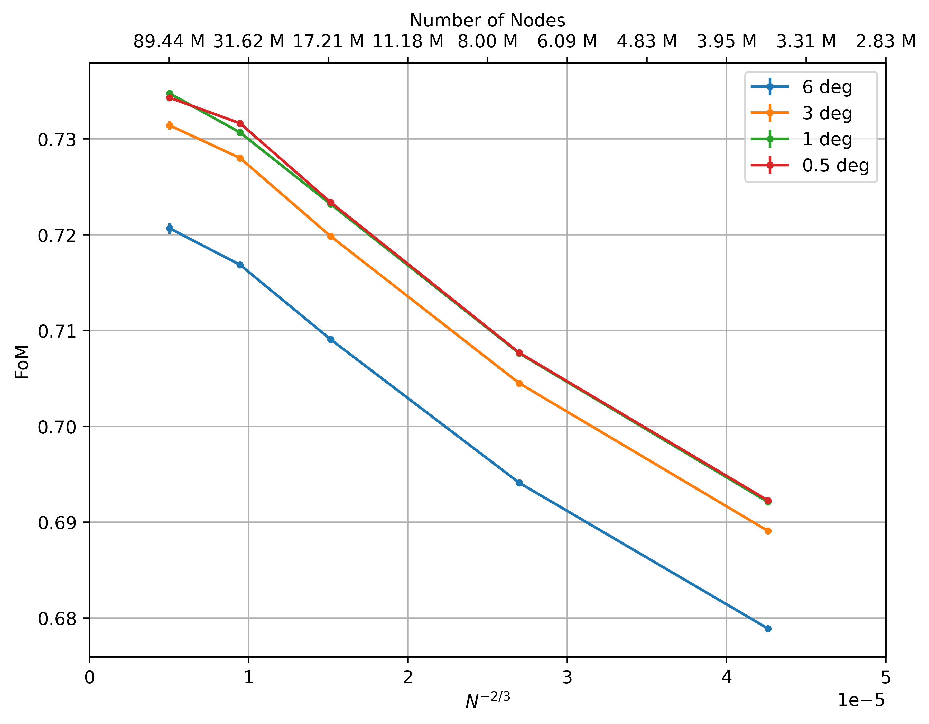
The first aspect worth highlighting is the close to negligible error bars for the integrated loads for the isolated rotor computations (not shown). A mesh refinement study shows that as the mesh is refined, the thrust and torque converge (not shown here). The increase in the FoM values as the time step is refined is primarily due to decreased torque values at finer time steps with minor differences for the finest two time steps.
The results are examined in further detail to explain the behavior of the integrated loads with mesh refinement and reduction in time step.

The sectional loads show a strong sensitivity to mesh refinement (Figure 2). Refinement of the mesh leads to a significantly better resolved tip vortex that has a large impact on the sectional loading inboard and outboard of approximately r/R = 0.9. Inboard, the preceding tip vortex induces downwash leading to a reduction in the local sectional loading, whereas outboard the tip vortex induces upwash leading to an increase in the local sectional loading. With mesh refinement, the location at which the tip vortex starts to impact the local loading also moves further inboard. Mesh refinement also leads to a reduction in local torque along the entire blade, especially in the location of the tip vortex. This is an example of favorable Blade-Vortex Interaction.
Let us now visualize the wakes using the Q-criterion colored with Mach number, shown in Figure 3. The wake visualizations show a strong dependency of the mesh on the resolved flow features away from the blade, whereas the dependency on the blade surface is weak except at the very tip. For the coarsest mesh, the tip vortices are poorly resolved. They are smeared at first, and later “end” because the Q criterion drops below the threshold level chosen. The solution highly resembles a blade-element theory solution where only a wide vortex tube is visible. As the mesh is refined the vortices are better resolved. The highest quality 5%c mesh shows instabilities in the rotor wake, which are seen in high-fidelity solutions in the literature. The secondary structures are due to the interaction of the tip vortices with the shear layers; thin shear layers are not marked by the Q criterion, by design. These structures are partly generated by the grid, which is not cylindrical, but braids are a well-known physical feature of mixing layers between the principal vortices.

Installed Rotor Setup
Let us now present the results for the installed rotor configuration which contains a fuselage. The integrated loads convergence for this setup with mesh refinement and time step reduction is shown in Figure 4. Note the much larger error bars on the integrated load predictions compared to the isolated rotor case (Figure 1). The primary reason for this is the presence of non 4/rev components with long transients in the loads, meaning that more rotor revolutions are required to obtain tighter error bars as well as the low number of samples used in the error bar computation. The rotor FoM value increases strongly with mesh refinement, but the time-step effect is weaker. All values of FoM fall within 0.5-a-count for time steps below 3 degrees and refinement level below 10%c, showing high confidence in the fine mesh/fine time step results.
We also observed that the temporal convergence of the loads is much tighter for the isolated rotor than for the installed rotor. For instance, the FoM variation over 3 revolutions is less than 0.2 counts in FoM for the isolated rotor, while it is 0.5 counts in FoM for the installed rotor. This is because the isolated rotor does not have to interact with the fuselage, while the installed rotor does; see Figure 5. The “fountain” near the rotor axis is very noticeable, but is not very accurate when the hub itself is omitted. On the other hand, the distribution on the blade is quite close to that on the isolated rotor, although the pressure difference is clearly higher on the blade that is over the tail of the fuselage. The temporal oscillations in the loads for the installed rotor calculations are caused by vortex shedding from the fuselage. To reduce these errors, at least 20 revolutions should be simulated to obtain highly accurate integrated loads data.

Collective sweep study
We now present results from the collective sweep study. For the isolated rotor, we use the 5%c mesh with time steps of 0.5 degree, but for the installed rotor the time step is reduced to 0.25 degree. The study is performed at two blade tip Mach numbers, namely 0.58 and 0.65, and the results are compared to other CFD codes and experimental data in Figure 6.

The isolated rotor results show good agreement with experimental data and other CFD codes. Due to the nature of installed rotor calculations, however, this level of accuracy is deemed acceptable with values from longer averaging cycles to be obtained in the future.
Conclusions
In summary, we presented a rigorous mesh sensitivity and time step study for isolated and installed hovering rotor solutions, aiming to assess the level of discretization error sensitivity. Based on the results, a collective sweep was performed with the results compared to available experimental data and other CFD codes. We can conclude the following key points from our study:
- For isolated rotor solutions, 30-40 million nodes and a 1-degree time step are sufficient for engineering-level accuracy. There is evidence of second-order grid convergence.
- Finer time steps are needed for installed rotor simulations, and higher resolution solutions improve wake resolution but do not significantly improve performance predictions.
- Convergence for installed rotor simulations is more difficult due to slow transients and unsteady vortex shedding, resulting in higher uncertainties in load predictions.
- Unsteady DES-based simulations are necessary for accurate hover performance predictions, especially at high blade loading.
- Flow360 hover performance predictions are within 1 count of experimental data and 1-2 counts of other CFD codes.
- Fuselage download predictions are within 2% of reference data, with further investigation planned on statistical convergence requirements.
This concludes the series of articles we prepared on our simulation study of a hovering rotor. Stay tuned for more content from our CFD research efforts using Flow360!
If you’d like to learn more about CFD simulations, how to optimize them, or how to reduce your simulation time from weeks or days to hours or minutes, stop by our website at flexcompute.com or follow us on LinkedIn.
For the expanded version of the paper this content is derived from, click here.