This tutorial will show you how to use field projections to obtain electromagnetic field data far away from a structure with knowledge of only near-field data.

When projecting fields, geometric approximations can be invoked to allow computing fields far away from the structure quickly and with good accuracy, but in Tidy3D we can also turn these approximations off when projecting fields at intermediate distances away, which gives a lot of flexibility.

These field projections are particularly useful for eliminating the need to simulate large regions of empty space around a structure.

In this notebook, we will

show how to compute projected fields on your local machine after a simulation is run, or on our servers during the simulation run.
show how to extract various quantities related to projected fields such as fields in different coordinate systems, power, and radar cross section.
demonstrate how, when far field approximations are used, the fields can dynamically be re-projected to new distances without having to run a new simulation.
study when geometric far field approximations should and should not be invoked, depending on the projection distance and the geometry of the structure.
show how to set up projections for finite-sized objects (e.g., scattering at a sphere) vs. thin but large-area structures (e.g., metasurfaces).

Table of contents¶

Simulation setup
Far-field projector setup
Server-side far field projection
Downsampling the near fields to speed up projections
Spatial filtering of far fields via windowing of near fields
Coordinate system conversion, power computation
Re-projection to a new far field distance
Exact field projections without making the far-field approximation
Projection to a grid defined in reciprocal space
Some final notes

[1]:

# standard python imports
import numpy as np
import matplotlib.pyplot as plt

# tidy3d imports
import tidy3d as td
import tidy3d.web as web

Far Field for a Uniformly Illuminated Aperture ¶

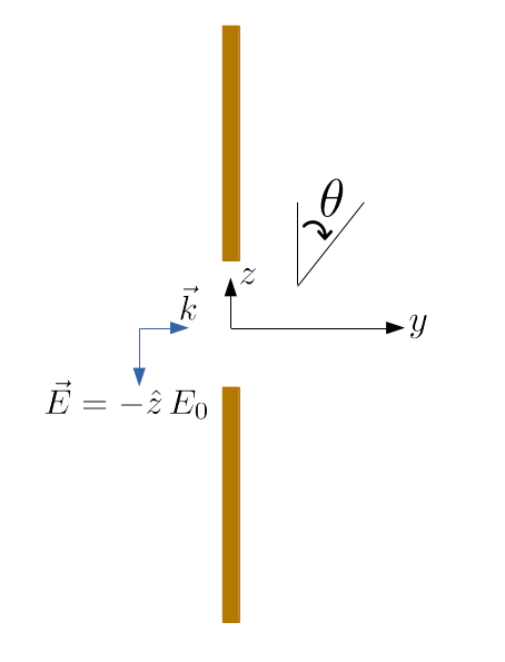
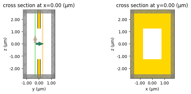
First, we will consider the simple case of an aperture in a perfect electric conductor sheet illuminated by a plane wave. The far fields in this case are known analytically, which allows for a straightforward comparison to Tidy3D's field projection functionality. We will show how to compute the far fields both on your local machine, and on the server. The geometry is shown below.

Geometry setup¶

[2]:

# size of the aperture (um)
width = 1.5
height = 2.5

# free space central wavelength (um)
wavelength = 0.75
# center frequency
f0 = td.C_0 / wavelength

# Define materials
air = td.Medium(permittivity=1)
pec = td.PECMedium()

# PEC plate thickness
thick = 0.2

# FDTD grid resolution
min_cells_per_wvl = 30

# create the PEC plate
plate = td.Structure(
    geometry=td.Box(size=[td.inf, thick, td.inf], center=[0, 0, 0]), medium=pec
)

# create the aperture in the plate
aperture = td.Structure(
    geometry=td.Box(size=[width, 1.5 * thick, height], center=[0, 0, 0]), medium=air
)

# make sure to append the aperture to the plate so that it overrides that region of the plate
geometry = [plate, aperture]

# define the boundaries as PML on all sides
boundary_spec = td.BoundarySpec.all_sides(boundary=td.PML())

# set the total domain size in x, y, and z
sim_size = [width * 2, 2, height * 2]

Source setup¶

For our incident field, we create a plane wave incident from the left, with the electric field polarized in the -z direction.

[3]:

# bandwidth in Hz
fwidth = f0 / 10.0

# time dependence of source
gaussian = td.GaussianPulse(freq0=f0, fwidth=fwidth)

# place the source to the left, propagating in the +y direction
offset_src = -0.3
source = td.PlaneWave(
    center=(0, offset_src, -0),
    size=(td.inf, 0, td.inf),
    source_time=gaussian,
    direction="+",
    pol_angle=np.pi / 2,
)

# Simulation run time
run_time = 50 / fwidth

Create monitor¶

First, we'll see how to do field projections using your machine after you've downloaded near fields from a Tidy3D simulation.

We create a surface FieldMonitor just to the right of the aperture to capture the near field data in the frequency domain.

We will turn off field colocation to obtain the raw data on the Yee grid. In the local field projection computation, fields are colocated internally as needed. In theory, turning off the server-side colocation avoids double interpolation in some cases. This can produce slightly more accurate results, although typically there should not be a significant difference.

[4]:

offset_mon = 0.3
monitor_near = td.FieldMonitor(
    center=[0, offset_mon, 0], size=[td.inf, 0, td.inf], freqs=[f0], name="near_field", colocate=False
)

Create Simulation¶

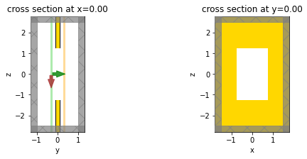
Now we can put everything together and define the simulation with a simple uniform mesh, and then we'll visualize the geometry to make sure everything looks right.

[5]:

sim = td.Simulation(
    size=sim_size,
    center=[0, 0, 0],
    grid_spec=td.GridSpec.uniform(dl=wavelength / min_cells_per_wvl),
    structures=geometry,
    sources=[source],
    monitors=[monitor_near],
    run_time=run_time,
    boundary_spec=boundary_spec,
)

fig, (ax1, ax2) = plt.subplots(1, 2, figsize=(9, 3))
sim.plot(x=0, ax=ax1)
sim.plot(y=0, ax=ax2)
plt.show();

No description has been provided for this image

Run simulation¶

[6]:

sim_data = web.run(
    sim, task_name="aperture_1", path="data/aperture_1.hdf5", verbose=True
)

12:27:48 EST Created task 'aperture_1' with task_id                             
             'fdve-9f87a07b-bb81-4408-9482-08e65924f548' and task_type 'FDTD'.

             View task using web UI at 'https://tidy3d.simulation.cloud/workbenc
             h?taskId=fdve-9f87a07b-bb81-4408-9482-08e65924f548'.

Output()

12:27:51 EST status = queued

Output()

12:28:19 EST status = preprocess

12:28:27 EST Maximum FlexCredit cost: 0.028. Use 'web.real_cost(task_id)' to get
             the billed FlexCredit cost after a simulation run.

             starting up solver

             running solver

             To cancel the simulation, use 'web.abort(task_id)' or              
             'web.delete(task_id)' or abort/delete the task in the web UI.      
             Terminating the Python script will not stop the job running on the 
             cloud.

Output()

12:28:36 EST early shutoff detected at 4%, exiting.

             status = postprocess

Output()

12:28:40 EST status = success

12:28:41 EST View simulation result at 'https://tidy3d.simulation.cloud/workbenc
             h?taskId=fdve-9f87a07b-bb81-4408-9482-08e65924f548'.

Output()

12:28:43 EST loading simulation from data/aperture_1.hdf5

Far field points ¶

Now, we'll define the set of observation angles far away from the source at which we'd like to measure the far fields.

[7]:

# radial distance away from the origin at which to project fields
r_proj = 50 * wavelength

# theta and phi angles at which to observe fields - part of the half-space to the right
theta_proj = np.linspace(np.pi / 10, np.pi - np.pi / 10, 100)
phi_proj = np.linspace(np.pi / 10, np.pi - np.pi / 10, 100)

Now, we define a far-field monitor, FieldProjectionAngleMonitor, which stores the information regarding the far field projection grid, and then we define the object that does the actual projections, FieldProjector.

[8]:

# far field projection monitor
monitor_far = td.FieldProjectionAngleMonitor(
    center=[
        0,
        offset_mon,
        0,
    ],  # the monitor's center defined the local origin - the projection distance
    # and angles will all be measured with respect to this local origin
    size=[td.inf, 0, td.inf],
    # the size and center of any far field monitor should indicate where the *near* fields are recorded
    freqs=[f0],
    name="far_field",
    phi=list(phi_proj),
    theta=list(theta_proj),
    proj_distance=r_proj,
    far_field_approx=True,  # we leave this to its default value of 'True' because we are interested in fields sufficiently
    # far away that geometric far field approximations can be invoked to speed up the calculation
)

# helper functin to call the projector
def get_proj_fields(sim_data, monitor_near, monitor_far, pts_per_wavelength=10):
    # object that does projections is constructed using the near-field monitor, because those are the fields to be projected
    projector = td.FieldProjector.from_near_field_monitors(
        sim_data=sim_data,
        near_monitors=[monitor_near],
        normal_dirs=["+"],  # we are projecting along the + direction
        pts_per_wavelength=pts_per_wavelength,  # to speed up calculations, the fields on the near-field monitor can be downsampled to these
        # many points per wavelength (default is already 10)
    )
    return projector.project_fields(monitor_far)


# execute the projector, with the far field monitor as input, to do the projection
# let's also time this, for later use
import time

t0 = time.perf_counter()
projected_field_data = get_proj_fields(sim_data, monitor_near, monitor_far)
t1 = time.perf_counter()
proj_time = t1 - t0

Output()

Analytical solution¶

Before we plot and analyze the results, we need reference data with which to perform comparisons. In our simple aperture example, an analytical expression for the far fields is already available, so we'll simply implement the analytic formula here at the observation points of interest.

[9]:

def analytic_fields_aperture(
    proj_monitor, sim_size, aperture_height, aperture_width, r_proj
):
    """Compute the far fields analytically."""
    # in Tidy3D, the plane wave source is normalized so that a total flux of 1 is injected into the simulation domain,
    # which corresponds to an electric field strength that is inversely proportional to the square root of the in-plane domain area
    thetas_ext = np.array(proj_monitor.theta)[None, :, None, None]
    phis_ext = np.array(proj_monitor.phi)[None, None, :, None]
    f = np.array(proj_monitor.freqs)[None, None, None, :]
    E0 = np.sqrt(2.0 * td.ETA_0 / sim_size[0] / sim_size[2])
    k = 2.0 * np.pi * f / td.C_0
    ux = k * np.sin(thetas_ext) * np.cos(phis_ext) * aperture_width / 2.0
    uz = k * np.cos(thetas_ext) * aperture_height / 2.0
    Etheta = -(
        -k
        / 2.0
        / np.pi
        / r_proj
        * E0
        * np.sin(thetas_ext)
        * np.exp(1j * k * r_proj)
        * aperture_height
        * aperture_width
        * np.sinc(ux / np.pi)
        * np.sinc(uz / np.pi)
    )
    Hphi = Etheta / td.ETA_0

    # for convenience, let's encapsulate the data into one of Tidy3D's native data structures designed for
    # storing far fields - this is the same format in which data will be returned when using Tidy3D's
    # 'FieldProjector', so comparisons will be easier to make
    coords = dict(
        r=np.array([r_proj]),
        theta=np.array(proj_monitor.theta),
        phi=np.array(proj_monitor.phi),
        f=np.array(proj_monitor.freqs),
    )
    Etheta_data = td.FieldProjectionAngleDataArray(Etheta, coords=coords)
    Hphi_data = td.FieldProjectionAngleDataArray(Hphi, coords=coords)
    Er_data = td.FieldProjectionAngleDataArray(np.zeros_like(Etheta), coords=coords)
    Ephi_data = td.FieldProjectionAngleDataArray(np.zeros_like(Etheta), coords=coords)
    Hr_data = td.FieldProjectionAngleDataArray(np.zeros_like(Etheta), coords=coords)
    Htheta_data = td.FieldProjectionAngleDataArray(np.zeros_like(Etheta), coords=coords)
    return td.FieldProjectionAngleData(
        monitor=proj_monitor,
        Er=Er_data,
        Etheta=Etheta_data,
        Ephi=Ephi_data,
        Hr=Hr_data,
        Htheta=Htheta_data,
        Hphi=Hphi_data,
        projection_surfaces=proj_monitor.projection_surfaces,
    )


analytic_field_data = analytic_fields_aperture(
    monitor_far, sim_size, height, width, r_proj
)

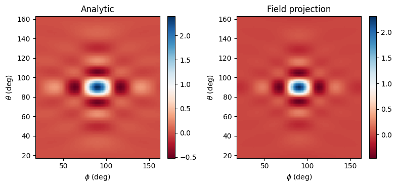
Plot and compare¶

Now we can compare the analytic fields to those computed via Tidy3D's FieldProjector, and also compute the root mean squared error between the two.

[10]:

def make_field_plot(phi, theta, vals1, vals2):
    n_plots = 2
    fig, ax = plt.subplots(1, n_plots, tight_layout=True, figsize=(8, 3.8))
    im1 = ax[0].pcolormesh(
        phi * 180 / np.pi,
        theta * 180 / np.pi,
        np.real(vals1),
        cmap="RdBu",
        shading="auto",
    )
    im2 = ax[1].pcolormesh(
        phi * 180 / np.pi,
        theta * 180 / np.pi,
        np.real(vals2),
        cmap="RdBu",
        shading="auto",
    )
    fig.colorbar(im1, ax=ax[0])
    fig.colorbar(im2, ax=ax[1])
    ax[0].set_title("Analytic")
    ax[1].set_title("Field projection")
    for _ax in ax:
        _ax.set_xlabel("$\phi$ (deg)")
        _ax.set_ylabel("$\\theta$ (deg)")


# RMSE
def rmse(array_ref, array_test):
    error = array_test - array_ref
    rmse = np.sqrt(np.mean(np.abs(error.flatten()) ** 2))
    nrmse = rmse / np.abs(np.max(array_ref.flatten()) - np.min(array_ref.flatten()))
    return nrmse


# plot Etheta
Etheta_analytic = analytic_field_data.Etheta.isel(f=0, r=0)
Etheta_proj = projected_field_data.Etheta.isel(f=0, r=0)
make_field_plot(phi_proj, theta_proj, Etheta_analytic, Etheta_proj)

# print the normalized RMSE
print(
    f"Normalized root mean squared error: {rmse(Etheta_analytic.values, Etheta_proj.values) * 100:.2f} %"
)

plt.show();

Normalized root mean squared error: 4.54 %

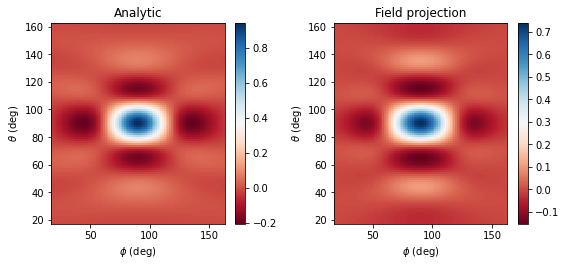
We obtain good agreement to analytical results. Now let's see if we can repeat this simulation but compute the far fields on the server, during the simulation run.

Server-side field projection ¶

All we have to do is provide the FieldProjectionAngleMonitor monitor as an input to the Tidy3D Simulation object as one of its monitors. Now, we no longer need to provide a separate near-field FieldMonitor - the near fields will automatically be recorded based on the size and location of the FieldProjectionAngleMonitor.

[11]:

sim2 = td.Simulation(
    size=sim_size,
    center=[0, 0, 0],
    grid_spec=td.GridSpec.uniform(dl=wavelength / min_cells_per_wvl),
    structures=geometry,
    sources=[source],
    monitors=[
        monitor_far
    ],  # just provide the far field FieldProjectionAngleMonitor as the input monitor
    run_time=run_time,
    boundary_spec=boundary_spec,
)

Run the new simulation.

[12]:

sim_data2 = web.run(
    sim2, task_name="aperture_2", path="data/aperture_2.hdf5", verbose=True
)

12:28:46 EST Created task 'aperture_2' with task_id                             
             'fdve-ab699c92-9bb1-4630-b1df-6705e6a92bd1' and task_type 'FDTD'.

             View task using web UI at 'https://tidy3d.simulation.cloud/workbenc
             h?taskId=fdve-ab699c92-9bb1-4630-b1df-6705e6a92bd1'.

Output()

12:28:48 EST status = queued

Output()

12:29:09 EST status = preprocess

12:29:16 EST Maximum FlexCredit cost: 0.028. Use 'web.real_cost(task_id)' to get
             the billed FlexCredit cost after a simulation run.

             starting up solver

12:29:17 EST running solver

             To cancel the simulation, use 'web.abort(task_id)' or              
             'web.delete(task_id)' or abort/delete the task in the web UI.      
             Terminating the Python script will not stop the job running on the 
             cloud.

Output()

12:29:25 EST early shutoff detected at 4%, exiting.

             status = postprocess

Output()

12:29:30 EST status = success

             View simulation result at 'https://tidy3d.simulation.cloud/workbenc
             h?taskId=fdve-ab699c92-9bb1-4630-b1df-6705e6a92bd1'.

Output()

12:29:32 EST loading simulation from data/aperture_2.hdf5

Now the projected fields are already contained in the returned sim_data2 object - all we have to do is access it as follows, and then plot and compare to analytical results as before.

[13]:

# extract the computed projected fields
projected_field_data_server = sim_data2[monitor_far.name]

# plot Etheta
Etheta_proj_server = projected_field_data_server.Etheta.isel(f=0, r=0)
make_field_plot(phi_proj, theta_proj, Etheta_analytic, Etheta_proj_server)

# print the normalized RMSE
print(
    f"Normalized root mean squared error: {rmse(Etheta_analytic.values, Etheta_proj_server.values) * 100:.2f} %"
)

plt.show();

Normalized root mean squared error: 4.54 %

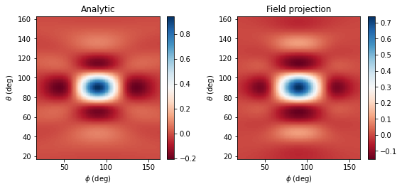
We obtain nearly identical results, except that they are computed much faster on our servers. Note also that in some cases, the server-side computations may be slightly more accurate than client-side ones, because on the server, the near fields are not downsampled at all.

To see the performance gains of using server-side computations, let's compare the time taken in each case.

[14]:

# use the simulation log to find the time taken for server-side computations
server_time = float(
    sim_data2.log.split("Field projection time (s):    ", 1)[1].split("\n", 1)[0]
)
print(f"Client-side field projection took {proj_time:.2f} s")
print(f"Server-side field projection took {server_time:.2f} s")

Client-side field projection took 2.73 s
Server-side field projection took 0.62 s

As expected, the server computes far fields faster than the local CPU-based computation, though it's a relatively small gain in this case. The gains in computation time are expected to be greater for larger and more complex setups.

Downsampling the near fields to speed up projections ¶

We can further speed up the server-side field projections by downsampling the near fields before projecting them to the far field. Typically, we should make sure that we are still sampling at least approximately 10 points per wavelength. Therefore, the downsampling feature is useful when the simulation resolution needs to be fairly high for the time stepping itself, but the projection step does not require such a high resolution.

All we have to do is provide the FieldProjectionAngleMonitor monitor (or any of the other field projection monitors) with an additional argument, interval_space, which defines the spatial interval at which to downsample the near fields. For example, a spatial interval of 2 implies that every 2nd near field point is used in the projection, which in turn means that roughly half the near field points are dropped. Note that the first and last points in the original grid are always kept in the near fields. We can downsample by a different amount along each direction.

[15]:

# make an updated copy of the projection monitor, this time requesting downsampling
monitor_far = monitor_far.copy(update={"interval_space": (4, 1, 3)}) # downsample by a factor of 4 along x, and 3 along y

# update the simulation object with this new monitor
sim2 = sim2.copy(update={"monitors": [monitor_far]})

Run the new simulation with downsampling

[16]:

sim_data2 = web.run(
    sim2, task_name="aperture_2", path="data/aperture_2.hdf5", verbose=True
)

             Created task 'aperture_2' with task_id                             
             'fdve-087b5a62-71fb-41db-ac84-d509e78b648c' and task_type 'FDTD'.

             View task using web UI at 'https://tidy3d.simulation.cloud/workbenc
             h?taskId=fdve-087b5a62-71fb-41db-ac84-d509e78b648c'.

Output()

12:29:34 EST status = queued

Output()

12:29:55 EST status = preprocess

12:30:04 EST Maximum FlexCredit cost: 0.028. Use 'web.real_cost(task_id)' to get
             the billed FlexCredit cost after a simulation run.

             starting up solver

             running solver

             To cancel the simulation, use 'web.abort(task_id)' or              
             'web.delete(task_id)' or abort/delete the task in the web UI.      
             Terminating the Python script will not stop the job running on the 
             cloud.

Output()

12:30:12 EST early shutoff detected at 4%, exiting.

12:30:13 EST status = postprocess

Output()

12:30:16 EST status = success

12:30:17 EST View simulation result at 'https://tidy3d.simulation.cloud/workbenc
             h?taskId=fdve-087b5a62-71fb-41db-ac84-d509e78b648c'.

Output()

12:30:18 EST loading simulation from data/aperture_2.hdf5

Now let's compare the downsampled projected fields to the analytical results

[17]:

# extract the computed projected fields
projected_field_data_server = sim_data2[monitor_far.name]

# plot Etheta
Etheta_proj_server = projected_field_data_server.Etheta.isel(f=0, r=0)
make_field_plot(phi_proj, theta_proj, Etheta_analytic, Etheta_proj_server)

# print the normalized RMSE
print(
    f"Normalized root mean squared error: {rmse(Etheta_analytic.values, Etheta_proj_server.values) * 100:.2f} %"
)

plt.show();

Normalized root mean squared error: 4.54 %

The results are virtually unaffected even though we used just a fraction of the data in the projection! Let's see how this changed the computation time, again compared to the client-side projection.

[18]:

# use the simulation log to find the time taken for server-side computations
server_time = float(
    sim_data2.log.split("Field projection time (s):    ", 1)[1].split("\n", 1)[0]
)
print(f"Client-side field projection took {proj_time:.2f} s")
print(f"Server-side field projection took {server_time:.2f} s")

Client-side field projection took 2.73 s
Server-side field projection took 0.57 s

The server-side projections are now faster than when we used all the data. Note that this is a fairly small problem, so the speed-up is marginal, but will be much more significant for larger problems.

Spatial filtering of far fields via windowing of near fields ¶

For surface field projection monitors, it is assumed that near fields go to zero near the edges of the near field monitor. In case the near fields do not go to zero, they are truncated, which can result in high-frequency artifacts in the far field. To alleviate these issues, we can apply a spatial filter via a Gaussian windowing function by specifying the window_size field in the FieldProjectionAngleMonitor monitor (or any of the other field projection monitors). This defines the size of the transition region over which the window is applied relative to half the size of the monitor, along each tangential direction. For more details, see the documentation here.

In the following, the windowing feature is demonstrated by repeating the aperture example from above for a larger aperture size, but using the window_size field instead of a physical PEC plate with a hole, to achieve an equivalent "aperture". The window_size field here was chosen based on trial and error.

[19]:

# size of the new larger aperture
new_aperture_width = width * 1.6
new_aperture_height = height * 1.6

# new projection monitor with windowing sizes chosen to approximate the physical aperture defined above
window_size = (0.37, 0.37)
new_monitor_far = monitor_far.copy(update={"window_size": window_size})

# new simulation object without a physical aperture, but with windowing enabled in the projection monitor
sim_window = sim.copy(update={
    "monitors": [new_monitor_far],
    "structures": [],
})

Run the new simulation

[20]:

sim_data_window = web.run(
    sim_window, task_name="aperture_2", path="data/aperture_2.hdf5", verbose=True
)

12:30:19 EST Created task 'aperture_2' with task_id                             
             'fdve-623c9da0-5e81-43b1-b9f5-06bcb8e1c127' and task_type 'FDTD'.

             View task using web UI at 'https://tidy3d.simulation.cloud/workbenc
             h?taskId=fdve-623c9da0-5e81-43b1-b9f5-06bcb8e1c127'.

Output()

12:30:21 EST status = queued

Output()

12:30:42 EST status = preprocess

12:30:51 EST Maximum FlexCredit cost: 0.028. Use 'web.real_cost(task_id)' to get
             the billed FlexCredit cost after a simulation run.

             starting up solver

             running solver

             To cancel the simulation, use 'web.abort(task_id)' or              
             'web.delete(task_id)' or abort/delete the task in the web UI.      
             Terminating the Python script will not stop the job running on the 
             cloud.

Output()

12:31:00 EST early shutoff detected at 4%, exiting.

             status = postprocess

Output()

12:31:03 EST status = success

             View simulation result at 'https://tidy3d.simulation.cloud/workbenc
             h?taskId=fdve-623c9da0-5e81-43b1-b9f5-06bcb8e1c127'.

Output()

12:31:05 EST loading simulation from data/aperture_2.hdf5

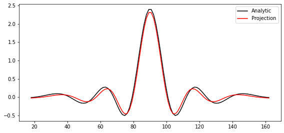
Plotting the results, we notice the excellent agreement between the analytical results for the aperture, and the projected fields resulting from windowing the near fields by an amount equivalent to an aperture of the given size.

[21]:

projected_data_window = sim_data_window[new_monitor_far.name]

# compute the analytic fields associated with the new window
analytic_field_data = analytic_fields_aperture(
    new_monitor_far, sim_size, new_aperture_height, new_aperture_width, r_proj
)

# plot the field distributions as before, in 2D and for a 1D slice at phi = pi / 2
Etheta_analytic = analytic_field_data.Etheta.isel(f=0, r=0)
Etheta_proj = projected_data_window.Etheta.isel(f=0, r=0)

fig, ax = plt.subplots(1, 1, tight_layout=True, figsize=(8, 3.8))
im1 = ax.plot(
    Etheta_analytic.theta * 180 / np.pi,
    np.real(Etheta_analytic.sel(phi=np.pi / 2, method="nearest")),
    '-k',
    label="Analytic",
)
im2 = ax.plot(
    Etheta_proj.theta * 180 / np.pi,
    np.real(Etheta_proj.sel(phi=np.pi / 2, method="nearest")),
    '-r',
    label="Projection",
)
ax.legend()

make_field_plot(phi_proj, theta_proj, Etheta_analytic, Etheta_proj)

# print the normalized RMSE
print(
    f"Normalized root mean squared error: {rmse(Etheta_analytic.values, Etheta_proj.values) * 100:.2f} %"
)

plt.show();

Normalized root mean squared error: 3.03 %

Other far field quantities and coordinate systems ¶

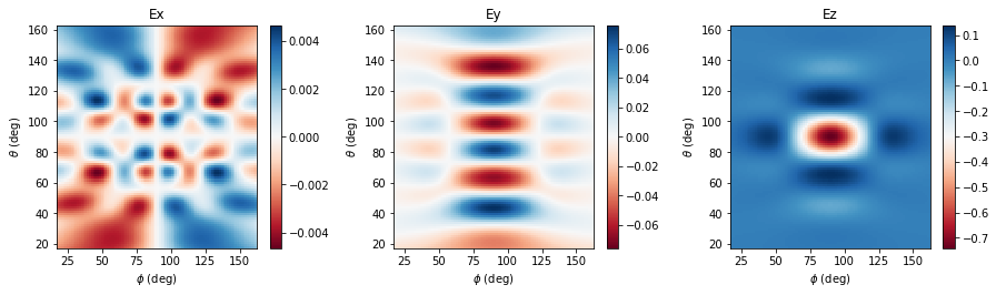
So far, we've been looking at the electric field in spherical coordinates. However, we can also look at the fields in other coordinate systems, e.g., E_x, E_y, E_z, and the radiated power, as follows:

[22]:

def make_cart_plot(phi, theta, vals1, vals2, vals3):
    n_plots = 3
    fig, ax = plt.subplots(1, n_plots, tight_layout=True, figsize=(12.6, 3.8))
    im1 = ax[0].pcolormesh(
        phi * 180 / np.pi,
        theta * 180 / np.pi,
        np.real(vals1),
        cmap="RdBu",
        shading="auto",
    )
    im2 = ax[1].pcolormesh(
        phi * 180 / np.pi,
        theta * 180 / np.pi,
        np.real(vals2),
        cmap="RdBu",
        shading="auto",
    )
    im3 = ax[2].pcolormesh(
        phi * 180 / np.pi,
        theta * 180 / np.pi,
        np.real(vals3),
        cmap="RdBu",
        shading="auto",
    )
    fig.colorbar(im1, ax=ax[0])
    fig.colorbar(im2, ax=ax[1])
    fig.colorbar(im3, ax=ax[2])
    ax[0].set_title("Ex")
    ax[1].set_title("Ey")
    ax[2].set_title("Ez")
    for _ax in ax:
        _ax.set_xlabel("$\phi$ (deg)")
        _ax.set_ylabel("$\\theta$ (deg)")


# get the fields in Cartesian coordinates from the projected data we already computed above
fields_cartesian = projected_field_data.fields_cartesian.isel(f=0, r=0)

# plot Ex, Ey, Ez
make_cart_plot(
    phi_proj, theta_proj, fields_cartesian.Ex, fields_cartesian.Ey, fields_cartesian.Ez
)

# get the power
power = projected_field_data.power.isel(f=0, r=0)

# plot the power
fig, ax = plt.subplots(1, 1, tight_layout=True, figsize=(4.3, 3.8))
im = ax.pcolormesh(
    phi_proj * 180 / np.pi,
    theta_proj * 180 / np.pi,
    power,
    cmap="inferno",
    shading="auto",
)
fig.colorbar(im, ax=ax)
_ = ax.set_title("Power")
_ = ax.set_xlabel("$\phi$ (deg)")
_ = ax.set_ylabel("$\\theta$ (deg)")

plt.show();

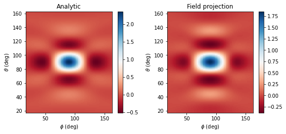
Re-projection to a different distance ¶

We can re-project the already-computed far fields to a different distance away from the structure - we neither need to run another simulation nor re-run the FieldProjector. Instead, the fields can simply be renormalized as shown below.

Note that by default, if no proj_distance was provided in the FieldProjectionAngleMonitor, the fields are projected to a distance of 1m.

[23]:

# new projection distance
r_proj_new = 20 * wavelength

# re-project our far field data above to this new distance
reprojected_field_data = projected_field_data.renormalize_fields(r_proj_new)

# now all the fields stored in 'projected_field_data' correspond to this new distance
# compare to the analytical fields at this new distance
analytic_field_data_new = analytic_fields_aperture(
    monitor_far, sim_size, height, width, r_proj_new
)

# plot Etheta
Etheta_analytic = analytic_field_data_new.Etheta.isel(f=0, r=0)
Etheta_proj = reprojected_field_data.Etheta.isel(f=0, r=0)
make_field_plot(phi_proj, theta_proj, Etheta_analytic, Etheta_proj)

# print the normalized RMSE
print(
    f"Normalized root mean squared error: {rmse(Etheta_analytic.values, Etheta_proj.values) * 100:.2f} %"
)

plt.show();

Normalized root mean squared error: 4.54 %

More accurate field projections ¶

In the field projections used above, the far field approximation is used: it is assumed that the fields are measured at a distance much greater than the size of our simulation in the transverse direction. Accordingly, geometric approximations are invoked, and any quantity whose magnitude drops off as 1/r^2 or faster is ignored. The advantages of these approximations are:

the projections are computed relatively fast
the projections are cast in a simple mathematical form which allows re-projecting the fields to different distance without the need to re-run a simulation or to re-run the FieldProjector.

However, in some cases we may want to project to intermediate distances where the far field approximation is no longer valid. Tidy3D's field projection functionality allows doing this very easily: simply flip a switch when defining the FieldProjectionAngleMonitor! The resulting computations will be a bit slower, but the results will be significantly more accurate.

Note: when the far field approximations are turned off, we can no longer simply use renormalize_fields to re-project the fields at a new distance. Instead, we would need to re-run the FieldProjector.

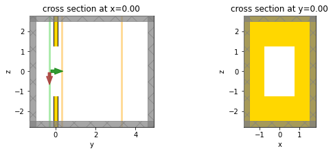
Below, we will demonstrate this feature by looking at fields only a few wavelengths away from the aperture. Note that our analytical results also made far field approximations, so here we'll make our simulation domain a bit larger and measure the actual fields on a monitor, so that we can compare these actual fields to those computed by the FieldProjector.

Also, this time we'll use the FieldProjectionCartesianMonitor, which is the counterpart to the FieldProjectionAngleMonitor where the observation grid is defined in Cartesian coordinates, not angles.

[24]:

# project fields only a few wavelengths away from the aperture
r_proj_intermediate = 4 * wavelength

# create a field monitor to measure these fields at the intermediate projection distance,
# so that we have something to which we can compare the 'FieldProjector' results
monitor_intermediate = td.FieldMonitor(
    center=[0, offset_mon + r_proj_intermediate, 0],
    size=[td.inf, 0, td.inf],
    freqs=[f0],
    name="inter_field",
)

# make a larger simulation along y to accommodate the plane at which the intermediate fields need to be measured
shift = 1.2 * r_proj_intermediate
sim_size3 = [sim_size[0], sim_size[1] + shift, sim_size[2]]
# move the sim center
sim_center = [0, (sim_size[1] + shift) / 2 - sim_size[1] / 2, 0]
sim3 = td.Simulation(
    size=sim_size3,
    center=sim_center,
    grid_spec=td.GridSpec.uniform(dl=wavelength / min_cells_per_wvl),
    structures=geometry,
    sources=[source],
    monitors=[
        monitor_near,
        monitor_intermediate,
    ],  # provide both near field and intermediate field monitors
    run_time=run_time,
    boundary_spec=boundary_spec,
)

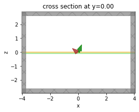
fig, (ax1, ax2) = plt.subplots(1, 2, figsize=(9, 3))
sim3.plot(x=0, ax=ax1)
sim3.plot(y=0, ax=ax2)
plt.show();

Run the new simulation.

[25]:

sim_data3 = web.run(
    sim3, task_name="aperture_3", path="data/aperture_3.hdf5", verbose=True
)

12:31:07 EST Created task 'aperture_3' with task_id                             
             'fdve-40454c45-9ab7-4941-9dc6-61fccf40573e' and task_type 'FDTD'.

             View task using web UI at 'https://tidy3d.simulation.cloud/workbenc
             h?taskId=fdve-40454c45-9ab7-4941-9dc6-61fccf40573e'.

Output()

12:31:09 EST status = queued

Output()

12:31:30 EST status = preprocess

12:31:38 EST Maximum FlexCredit cost: 0.065. Use 'web.real_cost(task_id)' to get
             the billed FlexCredit cost after a simulation run.

             starting up solver

             running solver

             To cancel the simulation, use 'web.abort(task_id)' or              
             'web.delete(task_id)' or abort/delete the task in the web UI.      
             Terminating the Python script will not stop the job running on the 
             cloud.

Output()

12:31:48 EST early shutoff detected at 8%, exiting.

             status = postprocess

Output()

12:31:53 EST status = success

             View simulation result at 'https://tidy3d.simulation.cloud/workbenc
             h?taskId=fdve-40454c45-9ab7-4941-9dc6-61fccf40573e'.

Output()

12:31:57 EST loading simulation from data/aperture_3.hdf5

Now let's create the FieldProjectionCartesianMonitor, this time turning off the far field approximations, and then run the FieldProjector again.

The FieldProjectionCartesianMonitor's xy observation grid is defined in a local coordinate system whose z axis points in the direction along which we want to project fields, in this case the +y axis. The mapping between local and global coordinates is as follows:

proj_axis=0: local x = global y, local y = global z
proj_axis=1: local x = global x, local y = global z
proj_axis=2: local x = global x, local y = global y

[26]:

# make the projection monitor which projects fields without approximations
xs = np.linspace(-sim_size[0] / 2, sim_size[0] / 2, 100)
ys = np.linspace(-sim_size[1] / 2, sim_size[1] / 2, 100)
monitor_intermediate_proj = td.FieldProjectionCartesianMonitor(
    center=[
        0,
        offset_mon,
        0,
    ],  # the monitor's center defined the local origin - the projection distance
    # and angles will all be measured with respect to this local origin
    size=[td.inf, 0, td.inf],
    freqs=[f0],
    name="inter_field_proj",
    proj_axis=1,  # because we're projecting along the +y axis
    x=list(xs),  # local x coordinates - corresponds to global x in this case
    y=list(ys),  # local y coordinates - corresponds to global z in this case
    proj_distance=r_proj_intermediate,
    far_field_approx=False,  # turn off the far-field approximation (is 'True' by default)
)

# execute the projector, with the projection field monitor as input, to do the projection
# let's also time this, for later use
import time

t0 = time.perf_counter()
projected_field_data_noapprox = get_proj_fields(
    sim_data3, monitor_near, monitor_intermediate_proj
)
t1 = time.perf_counter()
proj_time_new = t1 - t0

Output()

Now let's compare the following three results:

Directly-measured fields at the projection distance
Projected fields with approximations turned off
Projected fields with approximations turned on (just to compare the accuracy)

[27]:

# Compute projected fields *with* far field approximations, to facilitate an accuracy comparison
monitor_intermediate_proj_approx = td.FieldProjectionCartesianMonitor(
    center=[
        0,
        offset_mon,
        0,
    ],  # the monitor's center defined the local origin - the projection distance
    # and angles will all be measured with respect to this local origin
    size=[td.inf, 0, td.inf],
    freqs=[f0],
    name="inter_field_proj_approx",
    proj_axis=1,  # because we're projecting along the +y axis
    x=list(xs),  # local x coordinates - corresponds to global x in this case
    y=list(ys),  # local y coordinates - corresponds to global z in this case
    proj_distance=r_proj_intermediate,
    far_field_approx=True,  # turn on the far-field approximation
)

# execute the projector, with the projection field monitor as input, to do the projection
# let's also time this, for later use
import time

t0 = time.perf_counter()
projected_field_data_approx = get_proj_fields(
    sim_data3, monitor_near, monitor_intermediate_proj_approx
)
t1 = time.perf_counter()
proj_time_new_approx = t1 - t0

Output()

[28]:

# let's see how long this took compared to the previous case when the approximations were turned on
print(
    f"Client-side field projection *with approximations on* took {proj_time_new_approx:.2f} s"
)
print(
    f"Client-side field projection *with approximations off* took {proj_time_new:.2f} s"
)

Client-side field projection *with approximations on* took 5.95 s
Client-side field projection *with approximations off* took 13.23 s

As expected, when the approximations are turned off, the projections take longer. Now let's see if it was worth it!

[29]:

# Helper function to plot fields
def make_cart_plot(phi, theta, vals1, vals2, vals3):
    n_plots = 3
    fig, ax = plt.subplots(1, n_plots, tight_layout=True, figsize=(9, 3))
    im1 = ax[0].pcolormesh(ys, xs, np.real(vals1), cmap="RdBu", shading="auto")
    im2 = ax[1].pcolormesh(ys, xs, np.real(vals2), cmap="RdBu", shading="auto")
    im3 = ax[2].pcolormesh(ys, xs, np.real(vals3), cmap="RdBu", shading="auto")
    fig.colorbar(im1, ax=ax[0])
    fig.colorbar(im2, ax=ax[1])
    fig.colorbar(im3, ax=ax[2])
    ax[0].set_title("Ex")
    ax[1].set_title("Ey")
    ax[2].set_title("Ez")
    for _ax in ax:
        _ax.set_xlabel("$y$ (micron)")
        _ax.set_ylabel("$x$ (micron)")

[30]:

# plot the actual measured fields
fields_meas = sim_data3[monitor_intermediate.name].colocate(x=xs, z=ys)
make_cart_plot(
    ys,
    xs,
    fields_meas.Ex.isel(f=0, y=0),
    fields_meas.Ey.isel(f=0, y=0),
    fields_meas.Ez.isel(f=0, y=0),
)
plt.suptitle("Measured fields")

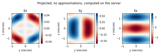
# projected field without approximations - get them in Cartesian coords
fields_proj_noapprox = projected_field_data_noapprox.fields_cartesian
make_cart_plot(
    ys,
    xs,
    fields_proj_noapprox.Ex.isel(f=0, y=0),
    fields_proj_noapprox.Ey.isel(f=0, y=0),
    fields_proj_noapprox.Ez.isel(f=0, y=0),
)
plt.suptitle("Projected, no approximations")

# projected field with approximations - get them in Cartesian coords
fields_proj_approx = projected_field_data_approx.fields_cartesian
make_cart_plot(
    ys,
    xs,
    fields_proj_approx.Ex.isel(f=0, y=0),
    fields_proj_approx.Ey.isel(f=0, y=0),
    fields_proj_approx.Ez.isel(f=0, y=0),
)
_ = plt.suptitle("Projected, with far field approximations")

# RMSE
Emag_meas = np.sqrt(
    np.abs(fields_meas.Ex) ** 2
    + np.abs(fields_meas.Ey) ** 2
    + np.abs(fields_meas.Ez) ** 2
)
Emag_proj_noapprox = np.sqrt(
    np.abs(fields_proj_noapprox.Ex) ** 2
    + np.abs(fields_proj_noapprox.Ey) ** 2
    + np.abs(fields_proj_noapprox.Ez) ** 2
)
Emag_proj_approx = np.sqrt(
    np.abs(fields_proj_approx.Ex) ** 2
    + np.abs(fields_proj_approx.Ey) ** 2
    + np.abs(fields_proj_approx.Ez) ** 2
)
print(
    f"Normalized RMSE for |E|, no far field approximation: {rmse(Emag_meas.values, Emag_proj_noapprox.values) * 100:.2f} %"
)
print(
    f"Normalized RMSE for |E|, with far field approximation: {rmse(Emag_meas.values, Emag_proj_approx.values) * 100:.2f} %"
)

plt.show();

12:32:16 EST WARNING: Colocating data that has already been colocated during the
             solver run. For most accurate results when colocating to custom    
             coordinates set 'Monitor.colocate' to 'False' to use the raw data  
             on the Yee grid and avoid double interpolation. Note: the default  
             value was changed to 'True' in Tidy3D version 2.4.0.

Normalized RMSE for |E|, no far field approximation: 0.43 %
Normalized RMSE for |E|, with far field approximation: 22.85 %

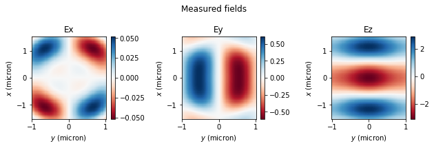
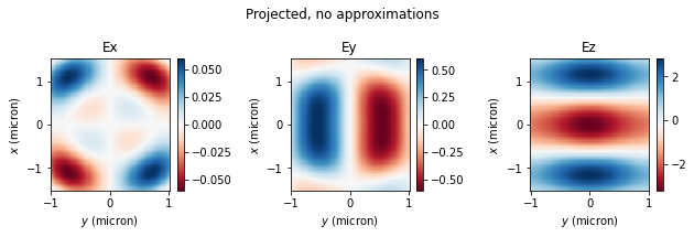
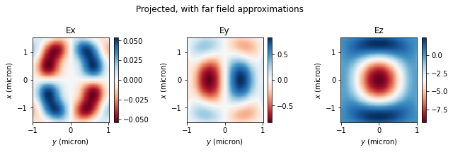
Without approximations, the projected fields match the measured ones extremely well! Instead, when approximations are used, the match is very poor. Thus, the accurate field projections can be extremely useful when the projection distance is not large compared to the structure size, but one still wants to avoid simulating all the empty space around the structure.

We should also note that this more accurate version of field projections can be run on the server in exactly the same way as before: just supply the projection monitor with its far_field_approx field set to False into the simulation's list of monitors as before. Everything else remains exactly the same, as shown below.

[31]:

sim4 = td.Simulation(
    size=sim_size,
    center=[0, 0, 0],
    grid_spec=td.GridSpec.uniform(dl=wavelength / min_cells_per_wvl),
    structures=geometry,
    sources=[source],
    monitors=[monitor_intermediate_proj],  # only need to supply the projection monitor
    run_time=run_time,
    boundary_spec=boundary_spec,
)

fig, (ax1, ax2) = plt.subplots(1, 2, figsize=(9, 3))
sim4.plot(x=0, ax=ax1)
sim4.plot(y=0, ax=ax2)
plt.show();

[32]:

# run the simulation
sim_data4 = web.run(
    sim4, task_name="aperture_4", path="data/aperture_4.hdf5", verbose=True
)

12:32:17 EST Created task 'aperture_4' with task_id                             
             'fdve-c98cd029-1ff9-470b-a61b-75004ddc810c' and task_type 'FDTD'.

             View task using web UI at 'https://tidy3d.simulation.cloud/workbenc
             h?taskId=fdve-c98cd029-1ff9-470b-a61b-75004ddc810c'.

Output()

12:32:19 EST status = queued

Output()

12:32:40 EST status = preprocess

12:32:46 EST Maximum FlexCredit cost: 0.028. Use 'web.real_cost(task_id)' to get
             the billed FlexCredit cost after a simulation run.

             starting up solver

12:32:47 EST running solver

             To cancel the simulation, use 'web.abort(task_id)' or              
             'web.delete(task_id)' or abort/delete the task in the web UI.      
             Terminating the Python script will not stop the job running on the 
             cloud.

Output()

12:32:55 EST early shutoff detected at 4%, exiting.

12:32:56 EST status = postprocess

Output()

12:32:59 EST status = success

             View simulation result at 'https://tidy3d.simulation.cloud/workbenc
             h?taskId=fdve-c98cd029-1ff9-470b-a61b-75004ddc810c'.

Output()

12:33:01 EST loading simulation from data/aperture_4.hdf5

[33]:

# extract the projected fields as before and plot them
projected_field_data_server = sim_data4[monitor_intermediate_proj.name]

# plot the actual measured fields from the previous simulation
fields_meas = sim_data3[monitor_intermediate.name].colocate(x=xs, z=ys)
make_cart_plot(
    ys,
    xs,
    fields_meas.Ex.isel(f=0, y=0),
    fields_meas.Ey.isel(f=0, y=0),
    fields_meas.Ez.isel(f=0, y=0),
)
plt.suptitle("Measured fields")

# projected field without approximations computed on the server
fields_proj_noapprox = projected_field_data_server.fields_cartesian
make_cart_plot(
    ys,
    xs,
    fields_proj_noapprox.Ex.isel(f=0, y=0),
    fields_proj_noapprox.Ey.isel(f=0, y=0),
    fields_proj_noapprox.Ez.isel(f=0, y=0),
)
plt.suptitle("Projected, no approximations, computed on the server")

# RMSE
Emag_proj_server = np.sqrt(
    np.abs(fields_proj_noapprox.Ex) ** 2
    + np.abs(fields_proj_noapprox.Ey) ** 2
    + np.abs(fields_proj_noapprox.Ez) ** 2
)
print(
    f"Normalized RMSE for |E|, no far field approximation, computed on the server: {rmse(Emag_meas.values, Emag_proj_server.values) * 100:.2f} %\n"
)

# use the simulation log to find the time taken for server-side computations
server_time = float(
    sim_data4.log.split("Field projection time (s):    ", 1)[1].split("\n", 1)[0]
)
print(
    f"Client-side field projection *without approximations* took {proj_time_new:.2f} s"
)
print(f"Server-side field projection *without approximations* took {server_time:.2f} s")

plt.show();

             WARNING: Colocating data that has already been colocated during the
             solver run. For most accurate results when colocating to custom    
             coordinates set 'Monitor.colocate' to 'False' to use the raw data  
             on the Yee grid and avoid double interpolation. Note: the default  
             value was changed to 'True' in Tidy3D version 2.4.0.

Normalized RMSE for |E|, no far field approximation, computed on the server: 0.28 %

Client-side field projection *without approximations* took 13.23 s
Server-side field projection *without approximations* took 0.92 s

Again we get an excellent match, an even smaller error than the client-side computations, and over an order of magnitude speed-up!

Reciprocal space monitor ¶

In addition to FieldProjectionAngleMonitor and FieldProjectionCartesianMonitor, one can also define the far field observation grid in reciprocal space using FieldProjectionKSpaceMonitor.

To demonstrate, we'll compute the far field associated with a Gaussian beam propagating at an angle.

[34]:

# create the Gaussian beam source positioned the same as the plane wave source above
gaussian_beam = td.GaussianBeam(
    center=(0, 0, -0.1 * wavelength),
    size=(td.inf, td.inf, 0),
    source_time=gaussian,
    direction="+",
    pol_angle=0,
    angle_theta=np.pi / 6,  # angles are with respect to the source plane's normal axis
    angle_phi=np.pi / 4,  # angles are with respect to the source plane's normal axis
    waist_radius=2 * wavelength,
    waist_distance=-wavelength * 4,
)

[35]:

# create the k-space far field projection monitor
monitor_far = td.FieldProjectionKSpaceMonitor(
    center=[0, 0, 0],
    size=[td.inf, td.inf, 0],
    freqs=[f0],
    name="far_field",
    ux=list(np.linspace(-0.7, 0.7, 100)),
    uy=list(np.linspace(-0.7, 0.7, 100)),
    proj_distance=50 * wavelength,
    proj_axis=2,  # projecting in the +y direction
    far_field_approx=True,  # use far field approximations
)

# create a simulation with the new source and monitor, and no PEC sheet
sim5 = td.Simulation(
    size=[10 * wavelength, 10 * wavelength, 7 * wavelength],
    center=[0, 0, 0],
    grid_spec=td.GridSpec.uniform(dl=wavelength / min_cells_per_wvl),
    structures=[],  # no PEC plate
    sources=[gaussian_beam],
    monitors=[monitor_far],
    run_time=run_time,
    boundary_spec=boundary_spec,
)

fig, (ax) = plt.subplots(1, 1, figsize=(7, 3))
sim5.plot(y=0, ax=ax)
plt.show();

Run simulation¶

[36]:

sim_data5 = web.run(
    sim5, task_name="kspace_monitor", path="data/kspace_monitor.hdf5", verbose=True
)

12:33:02 EST Created task 'kspace_monitor' with task_id                         
             'fdve-ef35642a-3ec2-404b-8026-6efe8853271d' and task_type 'FDTD'.

             View task using web UI at 'https://tidy3d.simulation.cloud/workbenc
             h?taskId=fdve-ef35642a-3ec2-404b-8026-6efe8853271d'.

Output()

12:33:04 EST status = queued

Output()

12:33:29 EST status = preprocess

12:33:33 EST Maximum FlexCredit cost: 0.198. Use 'web.real_cost(task_id)' to get
             the billed FlexCredit cost after a simulation run.

             starting up solver

12:33:34 EST running solver

             To cancel the simulation, use 'web.abort(task_id)' or              
             'web.delete(task_id)' or abort/delete the task in the web UI.      
             Terminating the Python script will not stop the job running on the 
             cloud.

Output()

12:33:48 EST early shutoff detected at 4%, exiting.

             status = postprocess

Output()

12:33:51 EST status = success

             View simulation result at 'https://tidy3d.simulation.cloud/workbenc
             h?taskId=fdve-ef35642a-3ec2-404b-8026-6efe8853271d'.

Output()

12:33:53 EST loading simulation from data/kspace_monitor.hdf5

Plot and compare¶

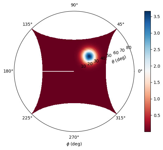
Extract and plot the fields. We use a polar plot, and observe that the far field spot is located along the phi=45 deg line, as expected. The angle theta is expected to be near 30 deg, which is nearly what is observed in the plot. The small deviation is due to the way the fields are plotted - a better way would be to project the fields orthographically on the surface of a sphere prior to plotting.

[37]:

# extract the computed projected fields
far_data = sim_data5[monitor_far.name]

# We can compute the theta and phi angles associated with the given reciprocal coordinates
coords = far_data.coords_spherical
theta = coords["theta"]
phi = coords["phi"]

# plot
Etheta = far_data.Etheta.isel(f=0, r=0)
fig, ax = plt.subplots(
    1, 1, tight_layout=True, figsize=(7, 5), subplot_kw={"projection": "polar"}
)
ax.grid(False)
# im = ax.pcolormesh(np.squeeze(phi), np.squeeze(theta) * 180 / np.pi, np.abs(Etheta), cmap='RdBu', shading='auto')
im = ax.pcolormesh(
    np.squeeze(phi),
    np.squeeze(theta) * 180 / np.pi,
    np.abs(Etheta),
    cmap="RdBu",
    shading="auto",
)
fig.colorbar(im, ax=ax)
_ = ax.set_xlabel("$\phi$ (deg)")

label_position = ax.get_rlabel_position()
_ = ax.text(
    np.radians(label_position - 8),
    ax.get_rmax() / 1.3,
    "$\\theta$ (deg)",
    rotation=label_position,
    ha="center",
    va="center",
)

plt.show();

/tmp/ipykernel_297577/2534941820.py:16: UserWarning: The input coordinates to pcolormesh are interpreted as cell centers, but are not monotonically increasing or decreasing. This may lead to incorrectly calculated cell edges, in which case, please supply explicit cell edges to pcolormesh.
  im = ax.pcolormesh(

Far Field for a Finite-Sized Structure¶

The above examples are very useful when simulating thin structure with a large extent in the lateral direction, such as a metasurface or metalens. If the structure is small enough, we may instead want to enclose it in a closed surface, which now serves as an equivalent surface in the spirit of the equivalence principle, without having to worry about whether the fields decay at the monitor's edges or not. To learn more, see the sphere radar cross section and plasmonic nanoparticle case studies.

Notes ¶

Since field projections rely on the surface equivalence principle, we have assumed that the tangential near fields recorded on the near field monitor serve as equivalent sources which generate the correct far fields. However, this requires that the field strength decays nearly to zero near the edges of the near-field monitor, which may not always be the case. For example, if we had used a larger aperture compared to the full simulation size in the transverse direction, we may expect a degradation in accuracy of the field projections. Despite this limitation, the field projections are still remarkably accurate in realistic scenarios. For realistic case studies further demonstrating the accuracy of the field projections, see our metalens and zone plate case studies.
The field projections make use of the analytical homogeneous medium Green's function, which assumes that the fields are propagating in a homogeneous medium. Therefore, one should use PMLs / absorbers as boundary conditions in the part of the domain where fields are projected. For far field projections in the context of perdiodic boundary conditions, see the diffraction efficiency example which demonstrates the use of a DiffractionMonitor.
Server-side field projections will add to the monetary cost of the simulation. However, typically the far field projections have a very small computation cost compared to the FDTD simulation itself, so the increase in monetary cost should be negligibly small in most cases.

[ ]:

Learning Center

Performing near field to far field projections¶

Table of contents¶

Far Field for a Uniformly Illuminated Aperture ¶

Geometry setup¶

Source setup¶

Create monitor¶

Create Simulation¶

Run simulation¶

Far field points ¶

Analytical solution¶

Plot and compare¶

Server-side field projection ¶

Downsampling the near fields to speed up projections ¶

Spatial filtering of far fields via windowing of near fields ¶

Other far field quantities and coordinate systems ¶

Re-projection to a different distance ¶

More accurate field projections ¶

Reciprocal space monitor ¶

Run simulation¶

Plot and compare¶

Far Field for a Finite-Sized Structure¶

Notes ¶