Inverse Design in Photonics Lecture 3: Adjoint Optimization

So today we’ll to continue our discussion of inverse design in photonics by providing a real example of an optimization of a device as enabled by the adjoint variable method.

So as an example, to design a lens, one can imagine a mathematical objective function as the simulated intensity at the focal point. More specifically, to design a lens, one would like to find a structure that maximizes the intensity for a given incident wave. One starts with a given structure as parameterized by various variables describing the device, for example, the geometry or the dialect constant of the system. Then one computes the gradient, which describes how to vary the device in a way that improves its performance. With the gradient, one can then adjust each of the structural parameters slightly along the gradient direction to improve the performance and repeat this process until convergence. Thus, it is clear that the gradient calculation is a key step in this process. In the last lecture, we described a very efficient method for computing the gradient with respect to an arbitrarily large number of parameters with only two simulations, called the “adjoint method”. This method allows one to significantly speed up, and in many ways, enable the optimization of these structures using gradient descent. In this lecture, we will give an example of how this works in practice.

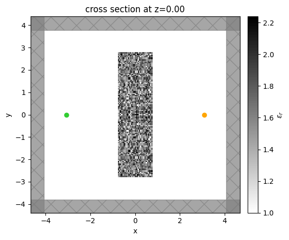
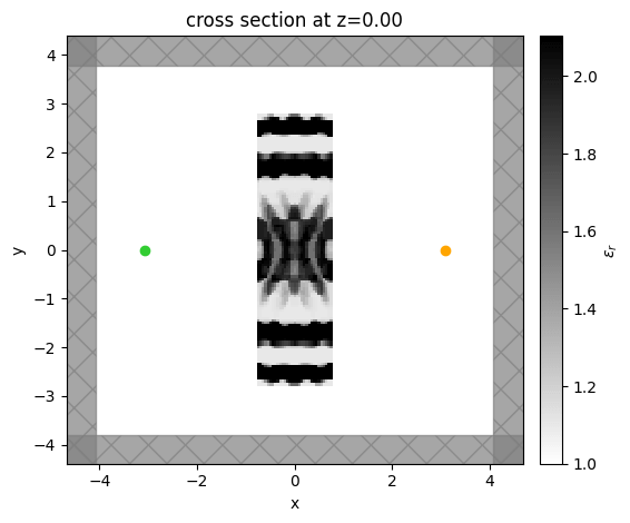
We start with a relatively simple example where our goal is to design a device to focus light. We imagine a two dimensional system with a point source as indicated by the green dot on the left. Our objective is to focus the emitted light from this point source as much as possible onto the orange point on the right, which indicates a field monitor. To accomplish this, we put a device in between the source and monitor as vacuum will not do this for you. Our problem thus becomes to design this device to maximize the focusing at the monitor location. We assume our device is described by a permittivity distribution within it’s rectangular region, which we can set arbitrarily to accomplish this objective.

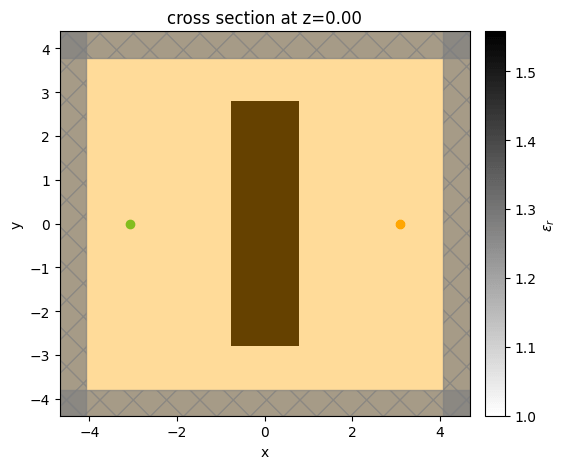
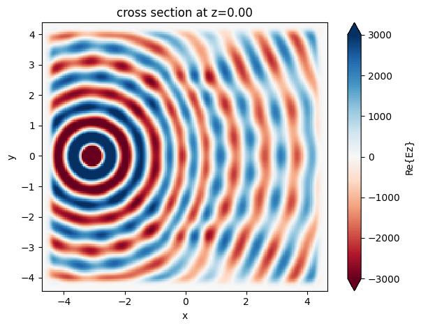
To start the optimization, we simply put a dielectric slab between the source and the monitor. The relative permittivity of this slab is 1.625, which is halfway between 1 (vacuum) and 2.25, which is a reasonable value for glass. In the middle panel, we show the starting electric field distribution, which shows (unsurprisingly) that the device does not focus at all. One can clearly see a cylindrical wave emanating from the point source and being perturbed a bit by the slab. Starting from this device, we iteratively update the device until it achieves focusing using the gradient information.

This slide shows the process of the full optimization algorithm as an animation. On the left is the permittivity distribution of our device at each iteration step, in the middle is the electric field corresponding to that permittivity distribution, and on the right is the intensity distribution. One can see that as we adjust the permittivity distribution inside the rectangle, the field pattern very quickly starts to exhibit this focusing behavior. This is particularly visible in the intensity distribution on the right hand side. So, in this kind of method, one can allow the computer to simply “figure out” what the optimum device configuration needs to be in order to achieve the functionality that you would like to accomplish. Now we will go into more detail about how this optimization is set up.

As mentioned, the design region here is inside of a rectangle between the point source and the measurement point. The first step is to break this design region into hundreds of pixels. We assume we can independently control the relative permittivity of the material at each of the pixels. Thus, these pixels define our design parameters that we can update during our optimization process. The adjoint variable method allows us to compute the gradient of the objective function with respect to each of these permittivity values using only two simulations! Note that there are quite a few practical considerations when setting up this optimization process, but we will talk more about these in subsequent lectures. Over the course of an optimization, one would therefore compute the gradient of the objective function with respect to the permittivity of each pixel and then update the values based on this gradient. However, there are not yet any constraints on the permittivity values, which is not realistic.

In practice, one only has control over a very small range of permittivity values. For example, if one is optimizing a glass-based structure, then the maximum permittivity one can get is the permittivity of glass (2.25). Therefore, it is useful to introduce a method to automatically constrain the permittivity to be within a minimum value and a maximum value to enable a structure that is more reasonable. For this purpose, instead of directly computing the gradient with respect to the permittivity, we constrain the permittivity between two bounds to the minimum and maximum by having an extra parameter “p” for each pixel that can span from negative infinity to positive infinity and smoothly maps to a permittivity value between our two bounds. In practice, we therefore compute the gradient with respect to these “p” values and update those in our optimization. The advantage of this approach is that you can be sure that the permittivity values of your device never extend outside of the allowed bounds.

With this parameterization, the optimization procedure is very similar to what we discussed previously regarding the relative permittivity. The only difference is that we compute the gradient with respect to the “p” parameters and update these “p” values directly.

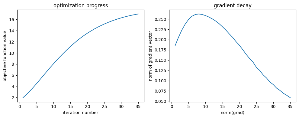
Here we show a few plots describing the optimization progress. On the left is the objective function as a function of the iteration number, recall this corresponds to the intensity at the measurement point. We see that the objective function steadily improves its ability to focus light. On the right, we show the norm of the gradient vector as a function of iteration step, which shows that the gradient is decaying as we reach a local maximum, which makes intuitive sense given our picture of the optimization procedure. Both of these plots give a strong indication that the gradient optimization is behaving exactly as one would expect.

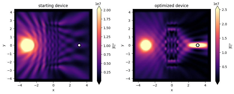
Lastly, we plot the final device and the corresponding intensity pattern. One can clearly see the focusing of the intensity at the monitor point. On the left, we show the dielectric structure that's generated by the computer, with a very unintuitive shape. You can see a distinctive variation, for example, along the y direction of the permittivity, which enables focusing. It is quite common that these optimization algorithms produce structures that are rather counter intuitive. In this case, one can imagine it is operating similar to a zone plate lens, but it is hard to intuitively understand how some of these final devices work in general. As a summary, in this lecture, we gave a first glimpse of how the gradient-based optimization enabled by the adjoint variable method works. There are many details that we will discuss in further lectures. One of the most important aspects is how to produce a final design that be fabricated, while we touched on this subject a little bit by constraining our permittivity values within a certain range, we will dedicate a lecture to this. Additionally, there are also many details regarding the optimization algorithm itself that are important to understand for improving performance, speed, and stability of the design process, which we will discuss further.